Time Series Analysis

Updated: 03 September 2023

Notes from the Complete Guide on Time Series Analysis in Python by Prashant Banerjee

Introduction

Time series analysis analyzes data over time to gain insights into the data in ways such as:

• Forecasting
• Signal Processing
• Pattern Recognition

Components of Time Series Data

• Trends - ancreasing, decreasing, or horizontal (stationary)
• Seasonality - a trend that repeats over time
• Cyclical Component - don’t necessarily have repeating trends but relate to actual correlations based on the nature of the time series data
• Irregular variation - Fluctuations that become visible when trends and cyclical variation is removed - may or may not be random
• ETS Decomposition - Error, Trend, and Seasonality - separate components of a time series

Types of Data

• Time series data - data collected over points in time
• Cross sectional data - Data of one or more variables recorded at the same point in time
• Pooled data - combination of the above

Terminology

• Dependence - association of two observations of the same variable
• Stationarity - mean value remains constant over time
• Differencing - make series stationary to control for auto-correlations
• Specification - testing the relationhips of variables
• Exponential smoothing - method used for short term predictions
• Curve fitting - regression done when data is non-linear
• ARIMA - Auto Regressive Integrated Moving Average

Patterns in Time Series

• A Trend is observed when there is an increasing or decreasing slope
• A Seasonality is observerd when there is a distinct repeated pattern at a specific frequency
• Cyclic behaviour occurs when the rise and fall is not a fixed frequency, this is different to seasonality

Not all data will have a trend and seasonality but should usually have one

Additive and Multiplicative Time Series

• Additive - $Value = Base + Trend + Seasonality + Error$
• Multiplicative = $Value = Base x Trend x Seasonality x Error$

Decomposition of a Time Series

Decomposition can be performed by considering the series asneither additive or multiplicative

Decomposition can be done using statsmodels like so:

1
from statsmodels.tsa.seasonal import seasonal_decompose
2

3
# For a monthly decomposition (period = 30)
4
multiplicative_decomposition = seasonal_decompose(df['Number of Passengers'], model='multiplicative', period=30)
5

6
additive_decomposition = seasonal_decompose(df['Number of Passengers'], model='additive', period=30)

The above can also be plotted using the plot method defined:

1
multiplicative_decomposition.plot()
2
additive_decomposition.plot()

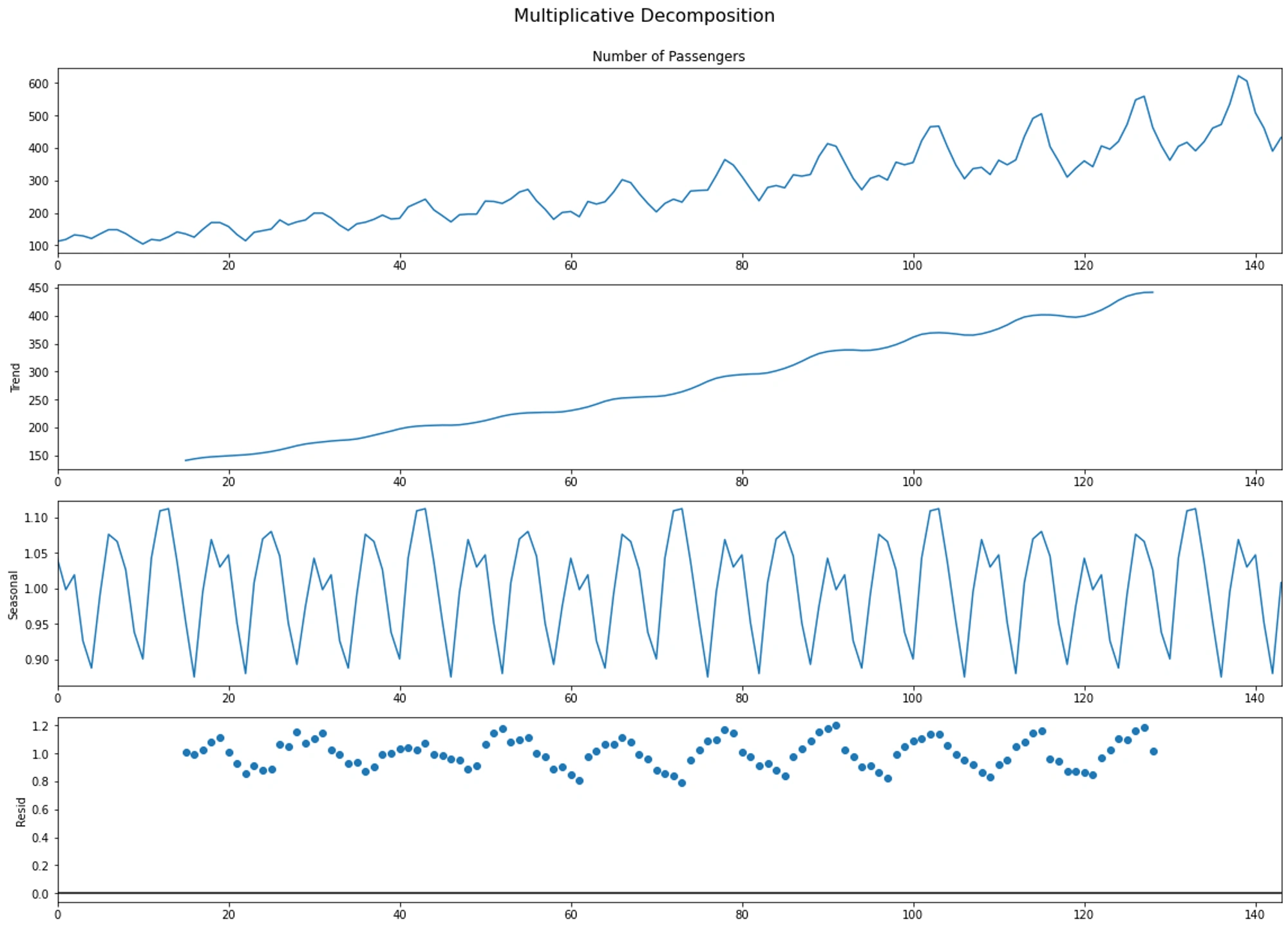
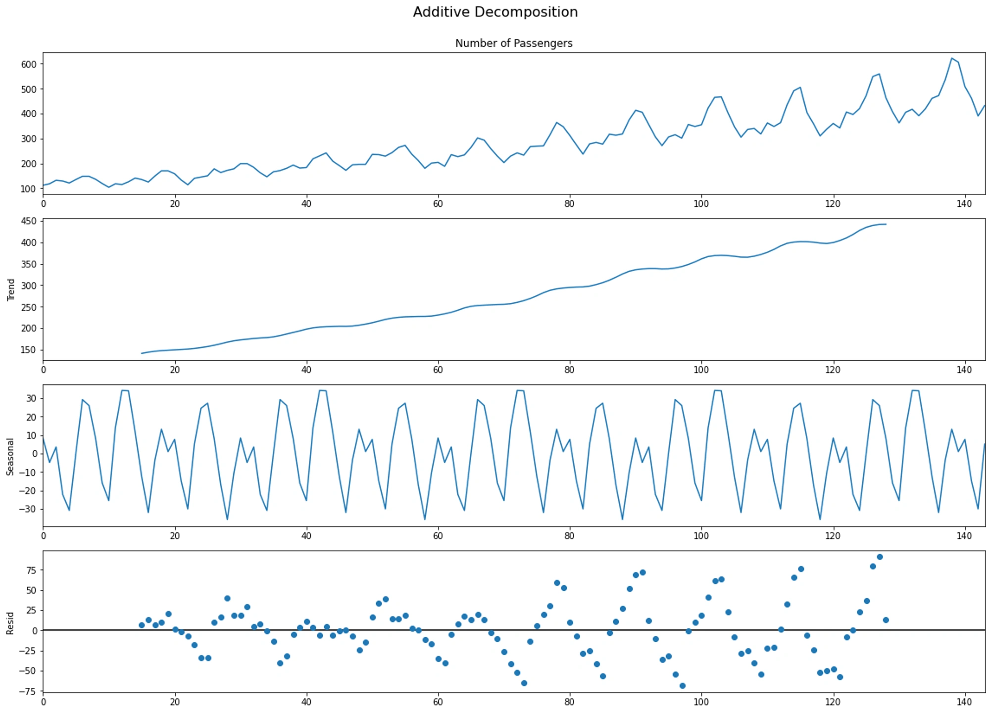
In the above series, comparing the additive and multiplicative residuals we can see that the additive one has some pattern left over whereas the risidual in the multiplicative is quite small and random, this tells us that the multiplicative decomposition is more appliccable to the series

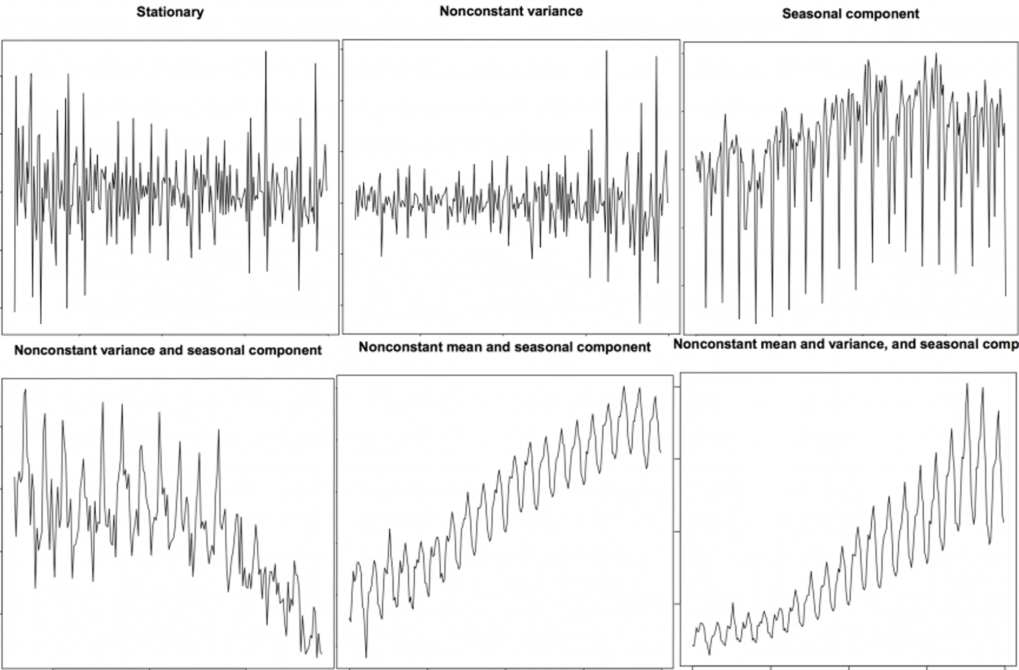
Stationary and Non-Stationary Time Series

A stationary series is one that is not a function of time, so values are independant of time

Statistical properties like mean, variance, and autocorrelation are constant over time - Auticorelation is a correlation of the series when compared to previous values

Stationary serieses are independant of seasonal effects

Below is a comparison of some stationary and non-stationary time series:

Making a Series Stationary

Why does a time series have to be stationary?

There are a few methods for making a series stationary

• Differencing
• Taking the Log
• Take the nth root
• Combination of the above

Differencing

Differencing is simply subtracting the previous value from the current value

The first difference may not make the series stationary, we can take further differences

Why Convert a Non-Stationary Series into a Stationary One Before Forecasting

• Forecasting a stationary series is relatively easy and moe reliable
• Autoregressive forecasting models are essentially linear regression models
• Stationarizing a series removes any persistent autocorrelation and makes predictors of the series nearly independent

Testing For Stationarity

• Look at a plot
• SPlit series into 2 or more contiguous parts and compute summary statistics (mean, variance, autocorrelation) - if these are similar then the series is likely stationary
• Unit root tests can be done on the series:
  • Augmented Dickey Fuller (ADF) test
  • Kwiatkowski-Phillips-Schmidt-Shin (KPSS) test (trend stationary)
  • Philips Perron (PP) test

Stationarity vs White Noise

White noise is not a function of time and also has a mean and variance that does not change over time

The difference between white noise and a stationarity is that white noise does not contain any resulting pattern

Detrend a Time Series

Detrending a time series means to remove the trend component which can be done using the following methods:

• Subtract the line of best fit
• Subtract the trend obtained from decomposition
• Subtract the mean
• Apply a filter like the Baxter-King filter (statsmodels.tsa.filters.bkfilter) or the Hodrick-Prescott Filter (statsmodels.tsa.filters.hpfilter)

Subtract the line of best fit

1
from scipy import signal
2

3
detrended = signal.detrend(df['Number of Passengers'].values)

Subtract the decomposition trend

1
from statsmodels.tsa.seasonal import seasonal_decompose
2
result_mul = seasonal_decompose(df['Number of Passengers'], model='multiplicative', period=30)
3
detrended = df['Number of Passengers'].values - result_mul.trend

Deseasonalize a Time Series

Some approaches for deseasonalizing a time series are as follows:

• Take a moving average with the length of the seasonal window
• Seasonal difference the series - subtract the previous season from the current one
• Divide the series by the seasonal index from the STL decomposition

If dividing does not work well we can also take a log of the series and then resotre by taking an exponential

1
# Time Series Decomposition
2
result_mul = seasonal_decompose(df['Number of Passengers'], model='multiplicative', period=30)
3

4
# Deseasonalize
5
deseasonalized = df['Number of Passengers'].values / result_mul.seasonal

Testing for Seasonality

To test for seasonality it can be simplest to plot the data, but if we want ot inspect this more specifically we can use an Autocorrelation Function (ACF) plot - if there is a strong seasonal pattern the ACF plot will shor repeated spikes at multiples of the seasonal window

Alternatively, a CHTest can also be used to determine if seasonal differencing is required

Autocorrelation and Partial Autocorrelation Functions

• Autocorrelation is a correlation of a series with its own lag. If ia series is significantly autocorrelated then it means that a previous series can help predict current value
• Partial Autocorrelation is a pure correlation of a series without contribution from intermediate lags

Autocorrelationa and Partial Autocorrelation can be found using statsmodels with the following code:

1
from statsmodels.tsa.stattools import acf, pacf
2
from statsmodels.graphics.tsaplots import plot_acf, plot_pacf
3

4
# Draw Plot
5
fig, axes = plt.subplots(1,2,figsize=(16,3), dpi= 100)
6
plot_acf(df['Number of Passengers'].tolist(), lags=50, ax=axes[0])
7
plot_pacf(df['Number of Passengers'].tolist(), lags=50, ax=axes[1])

Lag Plots

A lag plot is a scatter plot of a time series against a lag of itself and is used to check for autocorrelation. If there is any pattern in the series then the series is autocorrelated - if there is no pattern thatn the series is likel to be random

Granger Causality Test

Used to determine if one time series will be used to forecast another, it’s based on the idea that if X causes Y then forecast on Y based on previous values of X should outperform a forecast using only previuos values of Y

Smoothening a Time Series

Smoothening can be useful to:

• Reduce effect of noise
• Smootheened data can be used as a feature to explain the original series
• Visualize underlying trends

Some smoothening methods are:

• Take a moving average
• Do a LOESS smoothening (Localized regression)
• Do a LOWESS smoothening (Locally weighted regression)

Moving Average

An average of the rolling window, a large window will over-smooth a series

Localized regression

LOESS fits multiple regressions in the local neighborhood of each point