Time Series Forecasting
Time Series Forecasting using SKTime and SKLearn
Forecasting with SKTime
Resources
- Overview of time series analysis Python packages
- sktime - A Unified Toolbox for ML with Time Series - Markus Löning | PyData Global 2021
- GitHub SKTime Tutorial
# This Python 3 environment comes with many helpful analytics libraries installed
# It is defined by the kaggle/python Docker image: https://github.com/kaggle/docker-python
# For example, here's several helpful packages to load
# Input data files are available in the read-only "../input/" directory
# For example, running this (by clicking run or pressing Shift+Enter) will list all files under the input directory

import os
for dirname, _, filenames in os.walk('/kaggle/input'):
    for filename in filenames:
        print(os.path.join(dirname, filename))

# You can write up to 20GB to the current directory (/kaggle/working/) that gets preserved as output when you create a version using "Save & Run All"
# You can also write temporary files to /kaggle/temp/, but they won't be saved outside of the current session
!pip install sktime
!pip install pmdarima
import numpy as np
import pandas as pd
import seaborn as sns
import sktime as sktime
import matplotlib.pyplot as plt
The basic workflow when using SKTime is as follows:
- Specify data
- Specify task
- Specify model
- Fit
- Predict
SKTime also provides some sample datasets and other utilities under the sktime namespace:
from sktime.datasets import load_shampoo_sales
from sktime.utils.plotting import plot_series
df_shampoo = load_shampoo_sales()
plot_series(df_shampoo)
(<Figure size 1152x288 with 1 Axes>,
, <AxesSubplot:ylabel='Number of shampoo sales'>)
<Figure size 1152x288 with 1 Axes>

Forecasting
Forecasting works by taking the input data and trying to calculate what the data will be after X time period
This requires us to define a ForecastingHorizon which is the period of time over which we want to predict. sktime also has helpers for these
from sktime.forecasting.base import ForecastingHorizon
# timeframe to predict from
prediction_start = df_shampoo[-6:].index[0]

prediction_range = pd.period_range(prediction_start.start_time, freq=prediction_start.freqstr, periods=6)

prediction_range
PeriodIndex(['1993-07', '1993-08', '1993-09', '1993-10', '1993-11', '1993-12'], dtype='period[M]')
fh_shampoo = ForecastingHorizon(
    prediction_range,
    is_relative=False
)
train_cutoff = df_shampoo[-6:].index[0]

train_cutoff
Period('1993-07', 'M')
Train/Test Split
Splitting train and test data can be done by specifying the forecasting horizon, this will return a test set and train set where the test set is in the forecasting horizon
from sktime.forecasting.model_selection import temporal_train_test_split
y_train, y_test = temporal_train_test_split(df_shampoo, fh=fh_shampoo)
plot_series(y_train, y_test, labels=["y_train", "y_test"])
(<Figure size 1152x288 with 1 Axes>,
, <AxesSubplot:ylabel='Number of shampoo sales'>)
<Figure size 1152x288 with 1 Axes>

Forecasting Based on Test/Train Data
This is done similar to sklearn models:
- Instantiate model
- Fit model
- Predict
- Evaluate
To enable this methodology, sktime provides different forecasting models that can be used. Below is an example using a NaiveForecaster:
from sktime.forecasting.naive import NaiveForecaster
NaiveForecaster?
forecaster = NaiveForecaster(strategy="drift", window_length=10)
forecaster.fit(y_train)
NaiveForecaster(strategy='drift', window_length=10)
Once fitted, generate predictions using the ForecastingHorizon that was defined for the prediction period
y_pred = forecaster.predict(fh_shampoo)
plot_series(y_train, y_test, y_pred, labels=["y_train", "y_test", "y_pred"])
(<Figure size 1152x288 with 1 Axes>,
, <AxesSubplot:ylabel='Number of shampoo sales'>)
<Figure size 1152x288 with 1 Axes>

Model Evaluation
from sktime.performance_metrics.forecasting import mean_absolute_percentage_error
mean_absolute_percentage_error(y_test, y_pred)
0.16469764622516225
ARIMA Example
We can also use an ARIMA model for example as follows:
from sktime.forecasting.arima import AutoARIMA
# sp=12 for monthly data seasonality
forecaster = AutoARIMA(sp=12, suppress_warnings=True)
forecaster.fit(y_train)
AutoARIMA(sp=12, suppress_warnings=True)
y_pred = forecaster.predict(fh=fh_shampoo)
plot_series(y_train, y_test, y_pred, labels=["y_train", "y_test", "y_pred"])
(<Figure size 1152x288 with 1 Axes>,
, <AxesSubplot:ylabel='Number of shampoo sales'>)
<Figure size 1152x288 with 1 Axes>

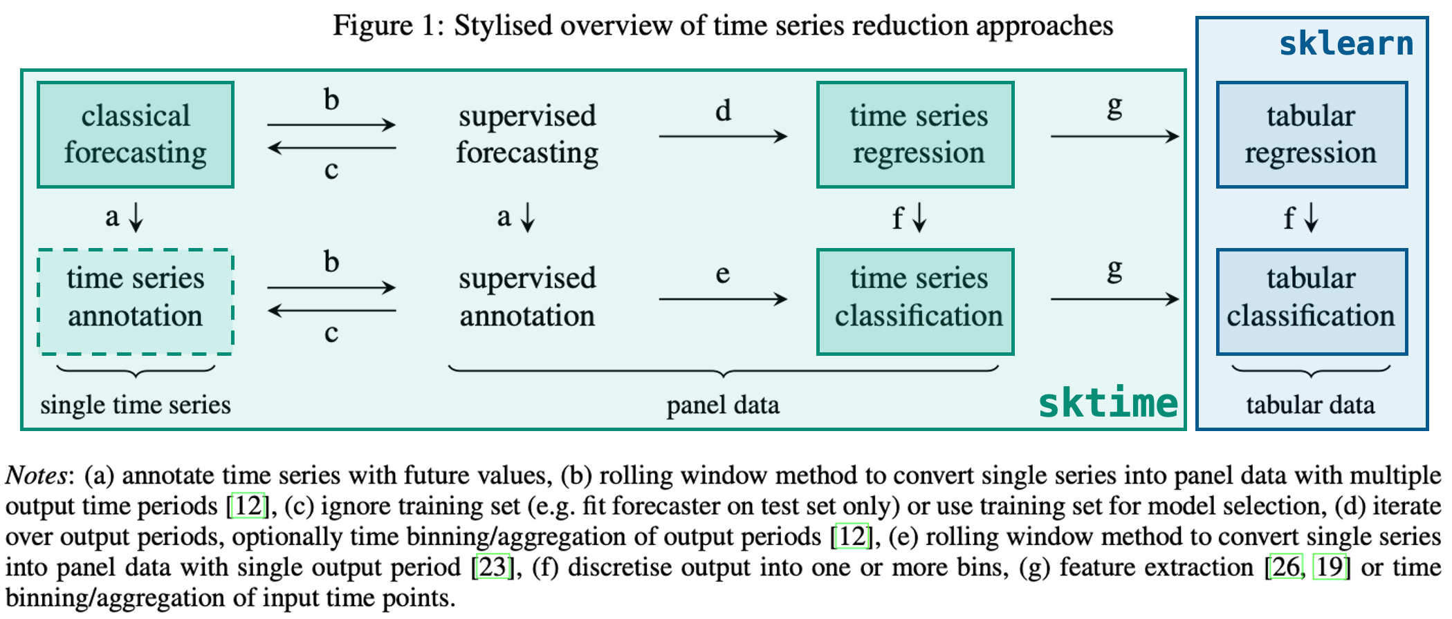
Using SKLearn Regressors
sktime also supports using sklearn regressors and supports transforming them into time-series compatible regressors by way of the make_reduction function:
from sklearn.neighbors import KNeighborsRegressor
from sktime.forecasting.compose import make_reduction

from sktime.datasets import load_airline
airline_df = load_airline()
y_train, y_test = temporal_train_test_split(airline_df, test_size=12)
plot_series(y_train, y_test, labels=["y_train", "y_test"])
(<Figure size 1152x288 with 1 Axes>,
, <AxesSubplot:ylabel='Number of airline passengers'>)
<Figure size 1152x288 with 1 Axes>

fh = ForecastingHorizon(y_test.index, is_relative=False)
transform a regressor into a forecaster
regressor = KNeighborsRegressor(n_neighbors=3)
forecaster = make_reduction(regressor, strategy="recursive", window_length=12)
forecaster.fit(y_train, fh=fh)
RecursiveTabularRegressionForecaster(estimator=KNeighborsRegressor(n_neighbors=3),
,                                     window_length=12)
y_pred = forecaster.predict(fh=fh)
plot_series(y_train, y_test, y_pred, labels=["y_train", "y_test", "y_pred"])
(<Figure size 1152x288 with 1 Axes>,
, <AxesSubplot:ylabel='Number of airline passengers'>)
<Figure size 1152x288 with 1 Axes>
