Introduction to Shaders
These notes and snippets are based/derived from The Book of Shaders by Patricio Gonzalez Vivo & Jen Lowe
Setup
For using these samples you will need some way to view shaders. I am using the glslCanvas VSCode extension for previewing shaders but you can also use another glslCanvas directly
Introduction
Fragment Shaders
Shaders are a set of instructions that are executed simultaneously for each pixel. Effectively, a fragment shader receives a position and returns a colour
Why are Shaders Fast
Shaders run on the GPU and are executed in parallel for each pixel on the screen. Since they run on the GPU they can take advantage of special hardware for speeding up matrix and trigonometric functions. In order to make this possible, there are some limitations imposed on them:
- Threads are "blind" to other threads - they cannot be dependent on each other
- Threads are "memoryless" - they do not have access to information about previous computations
GLSL
GLSL stands for "openGL Shading Language" and is one of the languages available for writing shaders
Hello World
THe hello world example for a shader looks like so:
#ifdef GL_ES
precision mediump float;
#endif

uniform float u_time;

void main(){
    gl_FragColor=vec4(0.,1.,1.,1.);
}
This example renders a simple colour to the screen. In the above we can see the following:
- A
mainfunction that is the entry point for the program - Builtin variables like
gl_FragColorwhich is the output color for the shader - Functions like
vec4which take in floats - The
vec4function takes in R,G,B,A channels as floats between 0 and 1 - Using floats between 0 and 1 is called normalizing and makes it easy for us to map vectors to different output spaces, e.g. color
- A preprocessor macro (
#ifdef ... #endif) which checks ifGL_ESis defined (which mostly happens when on mobile browsers) - The level of floating point precision to be used
precision mediump floatwhich sets the float prevision, this can also behighporlowp - Types are not cast and must be defined explicitly, so
1will not be automatically cast to the float1.0
Uniforms
Uniforms are data that is passed to our program from the CPU. Some of the uniforms taht are sent can be seen below:
uniform vec2 u_resolution;  // Canvas size (width,height)
uniform vec2 u_mouse;       // mouse position in screen pixels
uniform float u_time;       // Time in seconds since load
The uniform names and types may differ based on implementation, for example in ShaderToy they are as follows:
uniform vec3 iResolution;   // viewport resolution (in pixels)
uniform vec4 iMouse;        // mouse pixel coords. xy: current, zw: click
uniform float iTime;        // shader playback time (in seconds)
Using Uniforms
We can use uniforms just as any other variable, for example we can use the u_time uniform to set the color based on time:
#ifdef GL_ES
precision mediump float;
#endif

uniform vec2 u_resolution;// Canvas size (width,height)
uniform vec2 u_mouse;// mouse position in screen pixels
uniform float u_time;// Time in seconds since load

void main(){
    float variation=abs(sin(u_time));
    gl_FragColor=vec4(variation,0.,0.,1.);
}
We can also make use of the GPU accelerated functions like abs and sin. Some other GPU accelerated functions are sin(), cos(), tan(), asin(), acos(), atan(), pow(), exp(), log(), sqrt(), sign(), floor(), ceil(), fract(), mod(), min(), max(), and clamp()
gl_FragCoord
Another thing that is provided similar to gl_FragColor is gl_FragCoord which is the coordinates of the pixel or "screen fragment" that the current thread is working on.
Thegl_ variables are called "varying" and are different to uniforms which are the same across all threads
We can make use of this coordinate in the following code:
#ifdef GL_ES
precision mediump float;
#endif

uniform vec2 u_resolution;
uniform vec2 u_mouse;
uniform float u_time;

void main(){
    // Normalize the coordinate relative to resolution
    vec2 st=gl_FragCoord.xy/u_resolution;

    gl_FragColor=vec4(st.x,st.y,1.,1.);
}
Algorithmic Drawing
Shaping Functions
There are a few builtin shaping functions that we can use for creating a value that is varied based on some input parameter.
The simplest of these is the step function that returns a float that is either 0 if the value is less that the parameter, or 1 otherwise
#ifdef GL_ES
precision mediump float;
#endif

uniform vec2 u_resolution;
uniform vec2 u_mouse;
uniform float u_time;

void main(){
    vec2 st=gl_FragCoord.xy/u_resolution;

    float y=step(.5,st.x);
    vec3 color=vec3(y);

    gl_FragColor=vec4(color,1.);
}
There is also a smoothstep function that varies a value across the start and end ranges which can be used as follows:
#ifdef GL_ES
precision mediump float;
#endif

uniform vec2 u_resolution;
uniform vec2 u_mouse;
uniform float u_time;

void main(){
    vec2 st=gl_FragCoord.xy/u_resolution;

    float y=smoothstep(.3,.7,st.x);
    vec3 color=vec3(y);

    gl_FragColor=vec4(color,1.);
}
We can also use a combination of two smoothsteps that are slightly offset to create a line as follows:
float plot(vec2 st,float x){
    return
    smoothstep(x-.01,x,st.y)
    -smoothstep(x,x+.01,st.y);
}
We can then call this with the variable of interest to get an output value at the given point:
float y=abs(sin(st.x));
float plt=plot(st,y);
And we can then multiply the result by a color to actually view something:
vec3 color=plt*vec3(1.,0.,0.);
gl_FragColor=vec4(color,1.);
The result full code that renders a moving abs(sin(x)) for example can be seen below:
#ifdef GL_ES
precision mediump float;
#endif

uniform vec2 u_resolution;
uniform vec2 u_mouse;
uniform float u_time;

float plot(vec2 st,float x){
    return
    smoothstep(x-.01,x,st.y)
    -smoothstep(x,x+.01,st.y);
}

void main(){
    vec2 st=gl_FragCoord.xy/u_resolution;

    float y=abs(sin(st.x+u_time));

    float plt=plot(st,y);

    vec3 color=plt*vec3(0.,1.,1.);

    gl_FragColor=vec4(color,1.);
}
It's also possible to combine the lower level GLSL functions to get more complex mathematical functions, for example the below from Kynd
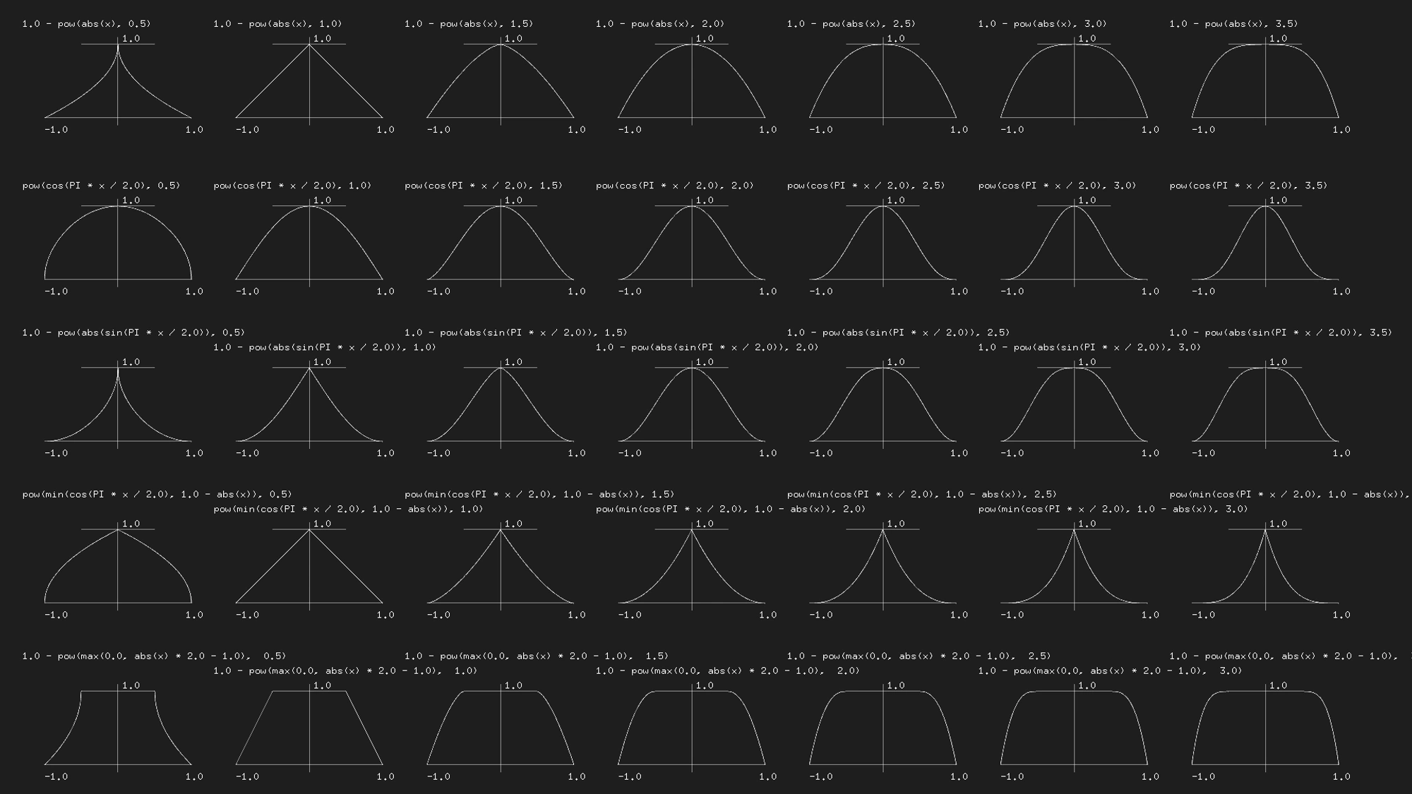
Additionally, the Lygia library also has a huge set of predefined shaping functions that you can use
Colors
Vectors
In general, we have been using colours using vec3 or vec4 vectors. We have mostly being accessing vector values using .x or .y, however there are a few different syntaxes that are equivalent
vec4 vector;
vector[0] = vector.r = vector.x = vector.s;
vector[1] = vector.g = vector.y = vector.t;
vector[2] = vector.b = vector.z = vector.p;
vector[3] = vector.a = vector.w = vector.q;
Furthermore, it's also possible to create new vectors out of vectors we and organize their parts as we want. For example:
vec4 color = vec4(1.,1.,0.,1.);

vec3 rgb = color.rgb;
vec3 rbg = color.rbg;
vec3 bgr = color.bgr;
vec3 bga = color.bga;
The above idea is called "swizzling" and can be applied to all vectors based on their components
Mixing Colors
Colors can be mixed using the mix function which can take a percentage value of how to mix the two colors. This can be seen below where we are using a sin wave based on the x coordinate and time to mix two colors:
#ifdef GL_ES
precision mediump float;
#endif

uniform vec2 u_resolution;
uniform vec2 u_mouse;
uniform float u_time;

void main(){
    vec2 st=gl_FragCoord.xy/u_resolution;

    float y=abs(sin(st.x+u_time));

    vec3 colorA=vec3(1.,1.,0.);
    vec3 colorB=vec3(0.,1.,1.);

    vec3 color=mix(colorA,colorB,y);

    gl_FragColor=vec4(color,1.);
}
HSB
There are multiple different ways that we can represent color. Using a function for converting from HSB to RGB we can render the colour space:
#ifdef GL_ES
precision mediump float;
#endif

uniform vec2 u_resolution;
uniform vec2 u_mouse;
uniform float u_time;

vec3 hsb2rgb(in vec3 c){
    vec3 rgb=clamp(abs(mod(c.x*6.+vec3(0.,4.,2.),6.)-3.)-1.,0.,1.);

    rgb=rgb*rgb*(3.-2.*rgb);
    return c.z*mix(vec3(1.),rgb,c.y);
}

void main(){
    vec2 st=gl_FragCoord.xy/u_resolution;

    float hue=st.x;
    float saturation=abs(sin(u_time));
    float brightness=st.y;

    vec3 color=hsb2rgb(vec3(hue,saturation,brightness));

    gl_FragColor=vec4(color,1.);
}
Since HSB is meant to be displayed as a polar color space, we can also display this as follows:
#ifdef GL_ES
precision mediump float;
#endif

#define TWO_PI 6.28318530718

uniform vec2 u_resolution;
uniform vec2 u_mouse;
uniform float u_time;

vec3 hsb2rgb(in vec3 c){
    vec3 rgb=clamp(abs(mod(c.x*6.+vec3(0.,4.,2.),6.)-3.)-1.,0.,1.);

    rgb=rgb*rgb*(3.-2.*rgb);
    return c.z*mix(vec3(1.),rgb,c.y);
}

void main(){
    vec2 st=gl_FragCoord.xy/u_resolution;

    vec2 toCenter=vec2(.5)-st;
    float angle=atan(toCenter.y,toCenter.x);
    float radius=length(toCenter)*2.;

    float hue=(angle/TWO_PI)+.5;
    float saturation=radius;

    vec3 color=hsb2rgb(vec3(hue,saturation,1.));

    gl_FragColor=vec4(color,1.);
}
Function Arguments
When defining functions we can define inputs as read only, write only, or read-write:
int newFunction(in vec4 aVec4,      // read-only
                out vec3 aVec3,     // write-only
                inout int aInt);    // read-write
Shapes
Rectangle
If we wanted to fill a rectangle in a shader, we need to think about how to determine the value for a single pixel, the general idea is as follows:
if (startX < x < endX) and (startY < y < endY)
    paint white
else
    paint black
When thinking about this from a shader standpoint, we can implement this kind of conditional using a step function
In our case, we need to do this in a few steps:
- Create the boundry for the left side, this is painting all content that is greater the left and bottom values:
float left=step(.1,st.x);// returns 1 when st.x > 0.1
float bottom=step(.1,st.y);// returns 1 when st.y > 0.1
- Create the boundary for right right and top sides by setting these back to white
float right=step(.1,1.-st.x);//returns 1 when (1-st.x) > 0.1
float top=step(.1,1.-st.y);//returns 1 when (1-st.x) > 0.1
- Multiplying the color components functions as a logical AND:
float pct = left * bottom * right * top;
vec3 color = vec3(pct);
Furthermore, we can simplify part 1. and 2. to use vectors directly instead of working with components, so the updated version for 1. and 2. combined looks like so:
vec2 bl=step(vec2(.1),st);
vec2 tr=step(vec2(.1),vec2(1.)-st);
Using the above, the final result can be seen below:
#ifdef GL_ES
precision mediump float;
#endif

uniform vec2 u_resolution;
uniform vec2 u_mouse;
uniform float u_time;

void main(){
    vec2 st=gl_FragCoord.xy/u_resolution.xy;

    vec2 bl=step(vec2(.1),st);
    vec2 tr=step(vec2(.1),vec2(1.)-st);

    float pct=bl.x*bl.y*tr.x*tr.y;
    vec3 color=vec3(pct);

    gl_FragColor=vec4(color,1.);
}
Circle
The approach for drawing a circle is a bit less confusing. Basically we define the distance of a point from a given location, in our case the center of the circle, and we use a step to include everything within that distance space:
#ifdef GL_ES
precision mediump float;
#endif

uniform vec2 u_resolution;
uniform vec2 u_mouse;
uniform float u_time;

void main(){
    vec2 st=gl_FragCoord.xy/u_resolution.xy;

    vec2 center=vec2(.5);

    float dist=distance(center,st);

    float pct=step(.5,1.-dist);
    vec3 color=vec3(pct);

    gl_FragColor=vec4(color,1.);
}
Distance Fields
The above implementation makes use of a distance field. A distance field tells us how far all the points in the field are from some reference point.
Note that the distance function uses the sqrt function underneath - this function can be computationally intensive so it can sometimes be more useful to define our operations without using the sqrt function in any way. For this example, it is also possible to implement a circle distance field using a smoothstep and the vector dot product which can be seen below:
#ifdef GL_ES
precision mediump float;
#endif

uniform vec2 u_resolution;
uniform vec2 u_mouse;
uniform float u_time;

void main(){
    vec2 st=gl_FragCoord.xy/u_resolution.xy;

    vec2 center=vec2(.5);
    float r=.5;

    vec2 dist=st-center;

    float pct=1.-smoothstep(r-(r*.01),r+(r*.01),dot(dist,dist)*4.);

    vec3 color=vec3(pct);

    gl_FragColor=vec4(color,1.);
}
Properties of Distance Fields
We can draw almost anything using distance fields. Once you have a formula to draw a specific shape using a distance field it becomes relatively easy to apply effects to it
We can visualize a distance field as the distance from the center to any given input point:
#ifdef GL_ES
precision mediump float;
#endif

uniform vec2 u_resolution;
uniform vec2 u_mouse;
uniform float u_time;

void main(){
    vec2 st=gl_FragCoord.xy/u_resolution.xy;

    vec2 center=vec2(.5);
    float dist=length(st-center);

    vec3 color=vec3(dist);

    gl_FragColor=vec4(color,1.);
}
Polar Shapes
Polar shapes depend on changing the distance of a circle. We can map catresian to polar coordinates using the following:
vec2 pos = vec2(0.5)-st;
float r = length(pos)*2.0;
float a = atan(pos.y,pos.x);
We can use these shapes along with the idea of using a smoothstep/step as a cutoff value to draw more complex shapes in combination with the polar coordinates:
#ifdef GL_ES
precision mediump float;
#endif

uniform vec2 u_resolution;
uniform vec2 u_mouse;
uniform float u_time;

void main(){
    vec2 st=gl_FragCoord.xy/u_resolution.xy;

    // get the polar coordinates
    vec2 pos=vec2(.5)-st;
    float r=length(pos)*2.;
    float a=atan(pos.y,pos.x);

    float f=sin(a*3.);

    vec3 color=vec3(1.-smoothstep(f,f+.01,r));

    gl_FragColor=vec4(color,1.);
}
Matrices
Once we know how to define specific shapes, we can use vector transformations to move them to different locations
Translation
The way we do this at the implementation level is by actually transforming the entire output coordinate space. We can see this by defining a new vector to move the space with below:
#ifdef GL_ES
precision mediump float;
#endif

uniform vec2 u_resolution;
uniform vec2 u_mouse;
uniform float u_time;

float circle(vec2 st,float r){
    vec2 center=vec2(.5);
    float dist=distance(center,st);
    float pct=step(1.-r,1.-dist);
    return pct;
}

void main(){
    vec2 st=gl_FragCoord.xy/u_resolution;

    vec2 translate=vec2(cos(u_time),sin(u_time*2.))*.3;

    st+=translate;

    float c=circle(st,.1);

    vec3 gradient=vec3(0.,st.x,st.y);
    vec3 color=gradient+vec3(c);

    gl_FragColor=vec4(color,1.);
}
If you observe the example above, you can see that it's not just the shape that moves but the entire color space. This is due to the coordinate system translation
2D Matrices
Doing more complex operations requires a matrix, for example we can translate as above by doing the dot product:
Rotation
For rotation, this is a bit more interesting
Using the above, we can implement the rotation as follows:
#ifdef GL_ES
precision mediump float;
#endif

uniform vec2 u_resolution;
uniform vec2 u_mouse;
uniform float u_time;

float rectangle(vec2 st,float x,float y){
    float b=step(.5-y*.5,st.y);
    float l=step(.5-x*.5,st.x);

    float t=step(.5-y*.5,1.-st.y);
    float r=step(.5-x*.5,1.-st.x);

    float pct=b*l*t*r;
    return pct;
}

vec2 rotate2d(vec2 st,in float theta){
    mat2 matrix=mat2(cos(theta),-sin(theta),
    sin(theta),cos(theta));

    vec2 trans=vec2(.5);

    // translate to the origin center
    st-=trans;

    // rotate
    st*=matrix;

    // move back to origin
    st+=trans;

    return st;
}

void main(){
    vec2 st=gl_FragCoord.xy/u_resolution;

    st=rotate2d(st,sin(u_time));

    float c=rectangle(st,.1,.1);

    vec3 gradient=vec3(0.,st.x,st.y);
    vec3 color=gradient+vec3(c);

    gl_FragColor=vec4(color,1.);
}
Scale
Similarly, we can define a matrix operation for scaling:
And the implementation of this can be seen below:
#ifdef GL_ES
precision mediump float;
#endif

uniform vec2 u_resolution;
uniform vec2 u_mouse;
uniform float u_time;

float circle(vec2 st,float r){
    vec2 center=vec2(.5);
    float dist=distance(center,st);
    float pct=step(1.-r,1.-dist);
    return pct;
}

vec2 scale(vec2 st,vec2 scale){
    mat2 matrix=mat2(
        scale.x,0.,
    0.,scale.y);

    vec2 trans=vec2(.5);

    st-=trans;
    st*=matrix;
    st+=trans;

    return st;
}

void main(){
    vec2 st=gl_FragCoord.xy/u_resolution;

    vec2 s=vec2(abs(sin(u_time)));
    st=scale(st,s);

    float c=circle(st,.1);

    vec3 gradient=vec3(0.,st.x,st.y);
    vec3 color=gradient+vec3(c);

    gl_FragColor=vec4(color,1.);
}
YUV Color
YUV is a color space for analog encoding of photos and videos that uses the human perception range.
We can define the conversions from YUV and RGB using a matrix and we can apply this to our input space to view the color range
#ifdef GL_ES
precision mediump float;
#endif

uniform vec2 u_resolution;
uniform vec2 u_mouse;
uniform float u_time;

mat3 yuv2rgb=mat3(1.,0.,1.13983,
    1.,-.39465,-.58060,
1.,2.03211,0.);

mat3 rgb2yuv=mat3(.2126,.7152,.0722,
    -.09991,-.33609,.43600,
.615,-.5586,-.05639);

void main(){
    vec2 st=gl_FragCoord.xy/u_resolution;

    // Remap our space since YUV goes from -1 to 1
    st-=.5;
    st*=2.;

    vec3 color=yuv2rgb*vec3(abs(sin(u_time)),st.x,st.y);

    gl_FragColor=vec4(color,1.);
}
Patterns
Since shaders execute once per pixel, no matter how much we repeat a shape the complexity is constant - this is a useful property for defining patterns
When creating patterns, we commonly use the fract function which gives us the decimal part of a number. Since our numbers are always between 1 and 0 this isn't instantly useful but becomes interesting when multiplying by some value
We can use this for displaying color:
#ifdef GL_ES
precision mediump float;
#endif

uniform vec2 u_resolution;
uniform vec2 u_mouse;
uniform float u_time;

void main(){
    vec2 st=gl_FragCoord.xy/u_resolution;

    st*=3.;
    st=fract(st);

    vec3 color=vec3(0,st.x,st.y);
    gl_FragColor=vec4(color,1.);
}
And we can do something similar using a circle:
#ifdef GL_ES
precision mediump float;
#endif

uniform vec2 u_resolution;
uniform vec2 u_mouse;
uniform float u_time;

float circle(vec2 st,float r){
    vec2 center=vec2(.5);
    float dist=distance(center,st);
    float pct=step(1.-r,1.-dist);
    return pct;
}

void main(){
    vec2 st=gl_FragCoord.xy/u_resolution;

    st*=3.;
    st=fract(st);

    float c=circle(st,.1);
    vec3 color=vec3(c);

    gl_FragColor=vec4(color,1.);
}
Since each subsection that we create above is a small sub-coordinate space, we can apply the other methods we've used to do stuff like rotate the space:
#ifdef GL_ES
precision mediump float;
#endif

uniform vec2 u_resolution;
uniform vec2 u_mouse;
uniform float u_time;

#define PI 3.14159265358979323846

float rectangle(vec2 st,float x,float y){
    float b=step(.5-y*.5,st.y);
    float l=step(.5-x*.5,st.x);

    float t=step(.5-y*.5,1.-st.y);
    float r=step(.5-x*.5,1.-st.x);

    float pct=b*l*t*r;
    return pct;
}

vec2 rotate2d(vec2 st,in float theta){
    mat2 matrix=mat2(cos(theta),-sin(theta),
    sin(theta),cos(theta));

    vec2 trans=vec2(.5);

    st-=trans;
    st*=matrix;
    st+=trans;

    return st;
}

void main(){
    vec2 st=gl_FragCoord.xy/u_resolution;

    st=rotate2d(st,PI*.25);

    st*=3.;
    st=fract(st);

    float c=rectangle(st,.5,.5);

    vec3 color=vec3(0.,1.,1.)*vec3(c);
    gl_FragColor=vec4(color,1.);
}
Or we can make use of the mod and step functions to identify which row we are in and translate that value halfway to the right like so:
#ifdef GL_ES
precision mediump float;
#endif

uniform vec2 u_resolution;
uniform vec2 u_mouse;
uniform float u_time;

float plot(vec2 st,float x){
    return
    smoothstep(x-.01,x,st.y)
    -smoothstep(x,x+.01,st.y);
}

float rectangle(vec2 st,float x,float y){
    float b=step(.5-y*.5,st.y);
    float l=step(.5-x*.5,st.x);

    float t=step(.5-y*.5,1.-st.y);
    float r=step(.5-x*.5,1.-st.x);

    float pct=b*l*t*r;
    return pct;
}

void main(){
    vec2 st=gl_FragCoord.xy/u_resolution;

    st*=5.;

    // returms 1. if we are in an odd numbered row
    float odd=step(1.,mod(st.y,2.));

    // shift the coordinate space by 0.5 if we are in an odd row
    st+=vec2(odd*.5,0.);

    // get the new fractional coordinate space
    st=fract(st);

    float c=rectangle(st,.5,.5);
    vec3 color=c*vec3(1.);

    gl_FragColor=vec4(color,1.);
}
Randomness
If we consider the function y = fract(sin(x)*n) we will notice that as we increase n at a certain point we get what looks like randomness:
#ifdef GL_ES
precision mediump float;
#endif

uniform vec2 u_resolution;
uniform vec2 u_mouse;
uniform float u_time;

float plot(vec2 st,float x){
    return
    smoothstep(x-.01,x,st.y)
    -smoothstep(x,x+.01,st.y);
}

void main(){
    vec2 st=gl_FragCoord.xy/u_resolution;

    float y=fract(sin(st.x)*1000000.);
    vec3 color=vec3(y);

    gl_FragColor=vec4(color,1.);
}
THe problem with using this kind of randomness is that while it is somewhat chaotic, it is not truly random since the underlying function is not random
Regardless, since we have a method of defining randomness, we can implement this in two dimensions as follows:
#ifdef GL_ES
precision mediump float;
#endif

uniform vec2 u_resolution;
uniform vec2 u_mouse;
uniform float u_time;

float random(vec2 st){
    float a=dot(st.xy,vec2(1000,1000));
    return fract(sin(a)*1000000.);
}

void main(){
    vec2 st=gl_FragCoord.xy/u_resolution;

    vec3 color=vec3(random(st));
    gl_FragColor=vec4(color,1.);
}
We do this by getting the dot product of the input vector and some other large vector and then using that to get the value that we pass to our pseudo random function
We can implement something interesting by combining this with the patterning/fraction method we learnt previously do get blocks of random colour instead of just noise:
#ifdef GL_ES
precision mediump float;
#endif

uniform vec2 u_resolution;
uniform vec2 u_mouse;
uniform float u_time;

#define TWO_PI 6.28318530718

float random(vec2 st){
    float a=dot(st.xy,vec2(74.61,20.53));
    return fract(sin(a)*83737.);
}

void main(){
    vec2 st=gl_FragCoord.xy/u_resolution;

    st*=10.;
    st=floor(st);

    vec3 color=vec3(random(st));
    gl_FragColor=vec4(color,1.);
}
This works since by getting the integer value (via the floor function) we effectively group our st.x and st.y values into buckets over a specified range
Next, we can use these values more directly by creting more complex patterns
#ifdef GL_ES
precision mediump float;
#endif

uniform vec2 u_resolution;
uniform vec2 u_mouse;
uniform float u_time;

#define TWO_PI 6.28318530718

float random(vec2 st){
    float a=dot(st.xy,vec2(74.61,20.53));
    return fract(sin(a)*83737.);
}

vec2 truchetPattern(in vec2 st,in float index){
    index=fract(((index-.5)*2.));
    if(index>.75){
        st=vec2(1.)-st;
    }else if(index>.5){
        st=vec2(1.-st.x,st.y);
    }else if(index>.25){
        st=1.-vec2(1.-st.x,st.y);
    }
    return st;
}

void main(){
    vec2 st=gl_FragCoord.xy/u_resolution;

    st*=10.;
    vec2 i=floor(st);

    st=fract(st);

    vec2 tile=truchetPattern(st,random(i));

    // sharp triangles
    // float c=step(tile.x,tile.y);

    // lines
    float c=smoothstep(tile.x,tile.x,tile.y)-
    smoothstep(tile.x,tile.x+.4,tile.y);

    vec3 color=vec3(c);

    gl_FragColor=vec4(color,1.);
}
Noise
Since very few things in nature are actually random but are a sort random with some sense of order. An example of a function that does something like this is ther Perlin noise algorithm and is a method for generating noise
Perlin Noise
This algorithm works by mixing the random values with other nearby noise values to create some kind of continuiy. There are of course different ways we can mix these values
For example, we can just use a plain mix:
#ifdef GL_ES
precision mediump float;
#endif

uniform vec2 u_resolution;
uniform vec2 u_mouse;
uniform float u_time;

float random(float x){
    return fract(sin(x)*1000000.);
}

float plot(vec2 st,float x){
    return
    smoothstep(x-.01,x,st.y)
    -smoothstep(x,x+.01,st.y);
}

float perlin(float steps,float x){
    x*=steps;
    float i=floor(x);
    float f=fract(x);

    return mix(random(i),random(i+1.),f);
}

void main(){
    vec2 st=gl_FragCoord.xy/u_resolution;

    float y=perlin(10.,st.x);

    vec3 color=vec3(plot(st,y));
    gl_FragColor=vec4(color,1.);
}
Or mixing using a smoothstep as well:
#ifdef GL_ES
precision mediump float;
#endif

uniform vec2 u_resolution;
uniform vec2 u_mouse;
uniform float u_time;

float plot(vec2 st,float x){
    return
    smoothstep(x-.01,x,st.y)
    -smoothstep(x,x+.01,st.y);
}

float random(float x){
    return fract(sin(x)*999999.);
}

float perlin(float steps,float x){
    x*=steps;
    float i=floor(x);
    float f=fract(x);

    return mix(random(i),random(i+1.),smoothstep(0.,1.,f));
}

void main(){
    vec2 st=gl_FragCoord.xy/u_resolution;

    float y=perlin(st.x,10.);

    vec3 color=vec3(plot(st,y));
    gl_FragColor=vec4(color,1.);
}
It is also possible to calculate your own custom curve instead of using something like smoothstep
#ifdef GL_ES
precision mediump float;
#endif

uniform vec2 u_resolution;
uniform vec2 u_mouse;
uniform float u_time;

float plot(vec2 st,float x){
    return
    smoothstep(x-.01,x,st.y)
    -smoothstep(x,x+.01,st.y);
}

float random(float x){
    return fract(sin(x)*1000000.);
}

float perlin(float steps,float x){
    x*=steps;
    float i=floor(x);
    float f=fract(x);

    // this is the same a as smoothstep
    float u=f*f*(3.-2.*f);

    return mix(random(i),random(i+1.),u);
}

void main(){
    vec2 st=gl_FragCoord.xy/u_resolution;

    float y=perlin(st.x,10.);

    vec3 color=vec3(plot(st,y));
    gl_FragColor=vec4(color,1.);
}
2D Noise
When doing 1D noise we interpolated between random values of x and x+1. For 2D noise however, we need to consider a plane with a point at each edge offset randomly
#ifdef GL_ES
precision mediump float;
#endif

uniform vec2 u_resolution;
uniform vec2 u_mouse;
uniform float u_time;

float random(in vec2 st){
    float a=dot(st.xy,vec2(9281.29,174.291));
    return fract(sin(a)*91287.);
}

float perlin(in vec2 st){
    vec2 i=floor(st);
    vec2 f=fract(st);

    // position 0,0
    float oo=random(i);

    // position 1,0
    float lo=random(i+vec2(1.,0.));

    // position 0,1
    float ol=random(i+vec2(0.,1.));

    // position 1,1
    float ll=random(i+vec2(1.,1.));

    vec2 u=smoothstep(vec2(0),vec2(1.),f);

    // mix the corner percentages
    return mix(oo,lo,u.x)+(ol-oo)*u.y*(1.-u.x)+
    (ll-lo)*u.x*u.y;
}

void main(){
    vec2 st=gl_FragCoord.xy/u_resolution;

    float y=perlin(st*5.);

    vec3 color=vec3(y);
    gl_FragColor=vec4(color,1.);
}
We can combine these ideas along with the methodology for working with polar coordinates and the user's mouse positon to do something kinda cool
Go ahead and try moving your mouse around on the image below
#ifdef GL_ES
precision mediump float;
#endif

uniform vec2 u_resolution;
uniform vec2 u_mouse;
uniform float u_time;

#define PI 3.14159265358979323846

float circle(vec2 st,float r){
    vec2 center=vec2(.5);
    float dist=distance(center,st);
    float pct=step(1.-r,1.-dist);
    return pct;
}

float angle(in vec2 v){
    vec2 pos=vec2(.5)-v;
    float r=length(pos)*2.;
    float a=atan(pos.y,pos.x);

    return a;
}

vec2 rotate(vec2 st,in float theta){
    mat2 matrix=mat2(cos(theta),-sin(theta),
    sin(theta),cos(theta));

    vec2 trans=vec2(.5);

    st-=trans;
    st*=matrix;
    st+=trans;

    return st;
}

float random(float x){
    return fract(sin(x)*1000000.);
}

float perlin(float steps,float x){
    x*=steps;
    float i=floor(x);
    float f=fract(x);

    return mix(random(i),random(i+1.),smoothstep(0.,1.,f));
}

vec2 shift(float a,float offset){
    vec2 dir=normalize(vec2((a),(a)));

    vec2 norm=dir;

    return norm*.1;
}

void main(){
    vec2 st=gl_FragCoord.xy/u_resolution;

    st=rotate(st,-PI/2.);

    float x=abs((u_mouse.x/u_resolution.x)-.5);
    float y=abs((u_mouse.y/u_resolution.y)-.5);
    float time=sin(u_time/5.)*10.;

    float r=.3+(x*.01);
    float sides=time;

    float a=abs(angle(st));
    float offset=perlin(sides,a)-.5;

    r+=offset*y*.3;
    vec3 color=vec3(circle(st,r+.005))-vec3(circle(st,r));

    gl_FragColor=vec4(color,1.);
}
Improving 2D Noise
Perlin noticed that in with the above noise method, it's possible to replace the smoothstep (cubic Hermite curve) with a quintic interpolation curve which maoes both ends of the curve more flat so that each border can stick more gracefully with the other enabling us to transition more smoothly between cells
Simplex Noise
Simplex noise improves upon the previous noise algorithms by accomplishing the following:
- Lower computational complexity and fewer multiplications
- Scales to higher dimensions with less computational cost
- No directional artifacts
- Well defined gradients
- Easy to implement in hardware
The simplex shape defined for a space with dimensions is . So for 2D noise we only need points, and for 3D noise we only need 4 points
Creating a simplex grid can be done by splitting a normal 4 cornered grid into two isosceles triangles and then skewing until the triangles are equilateral
We can see an example of skewing and subdividing this space below:
#ifdef GL_ES
precision mediump float;
#endif

uniform vec2 u_resolution;
uniform vec2 u_mouse;
uniform float u_time;

// Skew the X and Y Coordinates
vec2 skew(in vec2 st){
    float x=1.1547*st.x;
    float y=st.y+.5*x;

    return vec2(x,y);
}

// Subdivide a cell on the line x = y
vec2 subdivide(in vec2 st){
    vec2 result=vec2(0.);

    if(st.x>st.y){
        result=1.-vec2(st.x,st.y-st.x);
    }else{
        result=1.-vec2(st.x-st.y,st.y);
    }

    return fract(result);
}

void main(){
    vec2 st=gl_FragCoord.xy/u_resolution;

    st*=5.;
    st=skew(st);
    st=fract(st);
    st=subdivide(st);

    vec3 color=vec3(.3,st.x,st.y);
    gl_FragColor=vec4(color,1.);
}
This subdivision idea can be combined to create more powerful implementations of noise than the simple perlin case we have covered
Cellular Noise
Celllar noise is based on iterations. In GLSL we can iterate using loops but we must ensure that the number of loops we have is constant
Distance Field
Cellular Noise is based on distance fields. For each pixel we calculate the distance to the center of a cell, this means that we need to iterate through all our cells for a given pixel to find it's closest center
#ifdef GL_ES
precision mediump float;
#endif

uniform vec2 u_resolution;
uniform vec2 u_mouse;
uniform float u_time;

void main(){
    vec2 st=gl_FragCoord.xy/u_resolution;

    vec2 cells[5];
    cells[0]=vec2(.33,.25);
    cells[1]=vec2(.75,.25);
    cells[2]=vec2(.25,.75);
    cells[3]=vec2(.75,.75);
    cells[4]=u_mouse/u_resolution;

    float min_dist=1.;
    for(int i=0;i<5;i++){
        float dist=distance(st,cells[i]);
        min_dist=min(min_dist,dist);
    }

    vec3 color=vec3(min_dist);
    gl_FragColor=vec4(color,1.);
}
Tiling and iterations
For loops are not ideal for working with GLSL since we can't use dynamic exit limits and iterating significantly reduces the performance of a shader so this isn't really practical when using a large number of cells
We need to instead find a method that makes better use of the GPU
In order to do this, we can define a grid of 9 spaces around our current pixel, and check the value relative to that neighbor position since we don't need to evaluate non-neighboring grid members. Something like this:
for (int y= -1; y <= 1; y++) {
    for (int x= -1; x <= 1; x++) {
        // Neighbor place in the grid
        vec2 neighbor = vec2(float(x),float(y));
        ...
    }
}
We can use this to define a tiled cellular grid:
#ifdef GL_ES
precision mediump float;
#endif

uniform vec2 u_resolution;
uniform vec2 u_mouse;
uniform float u_time;

void main(){
    vec2 st=gl_FragCoord.xy/u_resolution;

    float grid=5.;

    st*=grid;
    vec2 i_st=floor(st);
    vec2 f_st=fract(st);

    float min_dist=1.;
    for(int y=-1;y<=1;y++){
        for(int x=-1;x<=1;x++){
            vec2 neighbor=i_st+vec2(float(x),float(y));
            float dist=distance(st,neighbor);
            min_dist=min(min_dist,dist);
        }
    }

    vec3 color=vec3(min_dist);
    gl_FragColor=vec4(color,1.);
}
Next, we can apply a random offset to the center point of each cell which will allow us to get something more interesting:
#ifdef GL_ES
precision mediump float;
#endif

uniform vec2 u_resolution;
uniform vec2 u_mouse;
uniform float u_time;

// Do some random stuff to get a 2d random value
vec2 random2d(vec2 p){
    return fract(vec2(dot(p*sin(p)*926000.,vec2(.6125,.222))));
}

void main(){
    vec2 st=gl_FragCoord.xy/u_resolution;

    float grid=5.;

    st*=grid;
    vec2 i_st=floor(st);
    vec2 f_st=fract(st);

    float min_dist=1.;
    for(int y=-1;y<=1;y++){
        for(int x=-1;x<=1;x++){
            // Get the root of the neighbor
            vec2 neighbor=vec2(float(x),float(y));

            // Define a center as the integer part + the neighbor
            // This will be the same for all values in a grid
            vec2 point=random2d(i_st+neighbor)+neighbor;

            // Get the distance from the neighbor's center the tile's center
            float dist=distance(f_st,point);

            // Store the distance to the closest centroid
            // This also compares with our current block's center
            min_dist=min(min_dist,dist);
        }
    }

    vec3 color=vec3(min_dist);
    gl_FragColor=vec4(color,1.);
}
Veronoi Algorithm
Instead of considering the algorithm from the perspective of the pixels as we have above, we can also take it from the perspectve of the point such that each point grows until it bumps nito another points - the algorithm for this is named after Georgy Veronoi
Creating veronoi diagrams from cellular noise involves keeping track of some additional information about the point which is closest to a pixel.
We will keep a reference to the center by storing a reference to the distance between our current point and the resolved center:
#ifdef GL_ES
precision mediump float;
#endif

uniform vec2 u_resolution;
uniform vec2 u_mouse;
uniform float u_time;

// do some random stuff to get a 2d random value
vec2 random2d(vec2 p){
    return fract(vec2(dot(p*sin(p)*926000.,vec2(.6125,.222))));
}

void main(){
    vec2 st=gl_FragCoord.xy/u_resolution;

    float grid=5.;

    st*=grid;
    vec2 i_st=floor(st);
    vec2 f_st=fract(st);

    float min_dist=1.;
    vec2 min_point=vec2(0.);

    for(int y=-1;y<=1;y++){
        for(int x=-1;x<=1;x++){
            vec2 neighbor=vec2(float(x),float(y));

            vec2 point=random2d(i_st+neighbor)+neighbor;

            float dist=distance(f_st,point);

            // store min point and distance
            if(dist<min_dist){
                min_dist=dist;
                min_point=point;
            }
        }
    }

    // make the min point relative to absolute coords
    min_point+=i_st;

    // color for cell
    vec2 cell_color=min_point/grid;
    vec3 color=cell_color.yxx;

    // Show color distance lines
    color-=abs(sin(50.*min_dist))*.05;

    gl_FragColor=vec4(color,1.);
}
Fractal Brownian Motion
A wave is a fluctuation of some property over time. Important aspects of a wave are it's amplitude and frequency
In the case of a wave, this is as follows:
Additionally, we can add waves up to create interference. This changes how the overall wave looks
#ifdef GL_ES
precision mediump float;
#endif

uniform vec2 u_resolution;
uniform vec2 u_mouse;
uniform float u_time;

float plot(vec2 st,float x){
    return
    smoothstep(x-.01,x,st.y)
    -smoothstep(x,x+.01,st.y);
}

void main(){
    vec2 st=gl_FragCoord.xy/u_resolution;
    st=st*6.-3.;

    float x=st.x;
    float t=u_time;

    float y=sin(x);

    // adding waves to create interference
    y+=sin(x*3.3+t*.125)*.12;
    y+=sin(x*4.4+t*.45)*.342;
    y+=sin(x*2.2+t*1.6)*.563;

    float plt=plot(st,y);

    vec3 color=plt*vec3(0.,1.,1.);

    gl_FragColor=vec4(color,1.);
}
We can use this idea to create noise based on this kind of interference to create something called fractal noise. for our case we'll use perlin noise instead of a sin wave:
#ifdef GL_ES
precision mediump float;
#endif

uniform vec2 u_resolution;
uniform vec2 u_mouse;
uniform float u_time;

float random(float x){
    return fract(sin(x)*1000000.);
}

float plot(vec2 st,float x){
    return
    smoothstep(x-.01,x,st.y)
    -smoothstep(x,x+.01,st.y);
}

float perlin(float x){
    float i=floor(x);
    float f=fract(x);

    return mix(random(i),random(i+1.),f);
}

void main(){
    vec2 st=gl_FragCoord.xy/u_resolution;
    st=st*4.-1.;

    float x=st.x;
    float t=u_time;

    float y=perlin(x);
    y+=perlin(x*3.3+t*.125)*.12;
    y+=perlin(x*4.4+t*.45)*.342;
    y+=perlin(x*2.2+t*1.6)*.563;

    float plt=plot(st,y);

    vec3 color=plt*vec3(0.,1.,1.);

    gl_FragColor=vec4(color,1.);
}
Fractal Brownian Motion
We can extend on this further by introducing a concept of octaves (iterations of noise), lacunarity (increments of frequency), and gain (amplitide) of the noise by which we apply variants of the same wave on top of itself
We can implement this using perlin noise as the base instead of a sin wave, our result is as follows:
#ifdef GL_ES
precision mediump float;
#endif

uniform vec2 u_resolution;
uniform vec2 u_mouse;
uniform float u_time;

float random(float x){
    return fract(sin(x)*999999.);
}

float plot(vec2 st,float x){
    return
    smoothstep(x-.01,x,st.y)
    -smoothstep(x,x+.01,st.y);
}

float perlin(float x){
    x*=5.;
    float i=floor(x);
    float f=fract(x);

    return mix(random(i),random(i+1.),smoothstep(0.,1.,f));
}

void main(){
    vec2 st=gl_FragCoord.xy/u_resolution;

    const int octaves=8;
    float lacunarity=2.;
    float gain=.5;

    float x=st.x;
    float t=u_time*.2;

    // initial values
    float amplitude=.5;
    float freq=1.;
    float y=0.;

    for(int i=0;i<octaves;i++){
        y+=amplitude*perlin(freq*x+t);
        freq*=lacunarity;
        amplitude*=gain;
    }

    float plt=plot(st,y);

    vec3 color=plt*vec3(0.,1.,1.);

    gl_FragColor=vec4(color,1.);
}
We can also implement something like this in two dimensions:
#ifdef GL_ES
precision mediump float;
#endif

uniform vec2 u_resolution;
uniform vec2 u_mouse;
uniform float u_time;

float random(in vec2 st){
    float a=dot(st.xy,vec2(12.29,1.291));
    return fract(sin(a)*1125163.);
}

float perlin(in vec2 st){
    vec2 i=floor(st);
    vec2 f=fract(st);

    float oo=random(i);
    float lo=random(i+vec2(1.,0.));
    float ol=random(i+vec2(0.,1.));
    float ll=random(i+vec2(1.,1.));

    vec2 u=smoothstep(vec2(0),vec2(1.),f);

    return mix(oo,lo,u.x)+(ol-oo)*u.y*(1.-u.x)+
    (ll-lo)*u.x*u.y;
}

float fbm(in vec2 st,float lacunarity,float gain){
    const int octaves=8;

    float t=u_time*.5;

    // initial values
    float amplitude=.5;
    float freq=4.;
    float r=0.;

    for(int i=0;i<octaves;i++){
        r+=amplitude*perlin(freq*st+t);
        freq*=lacunarity;
        amplitude*=gain;
    }

    return r;
}

void main(){
    vec2 st=gl_FragCoord.xy/u_resolution;

    float r=fbm(st,2.,.5);

    vec3 color=vec3(r);

    gl_FragColor=vec4(color,1.);
}