Data Science Methodology
Updated: 03 September 2023
Based on this Cognitive Class Course
The Methodology
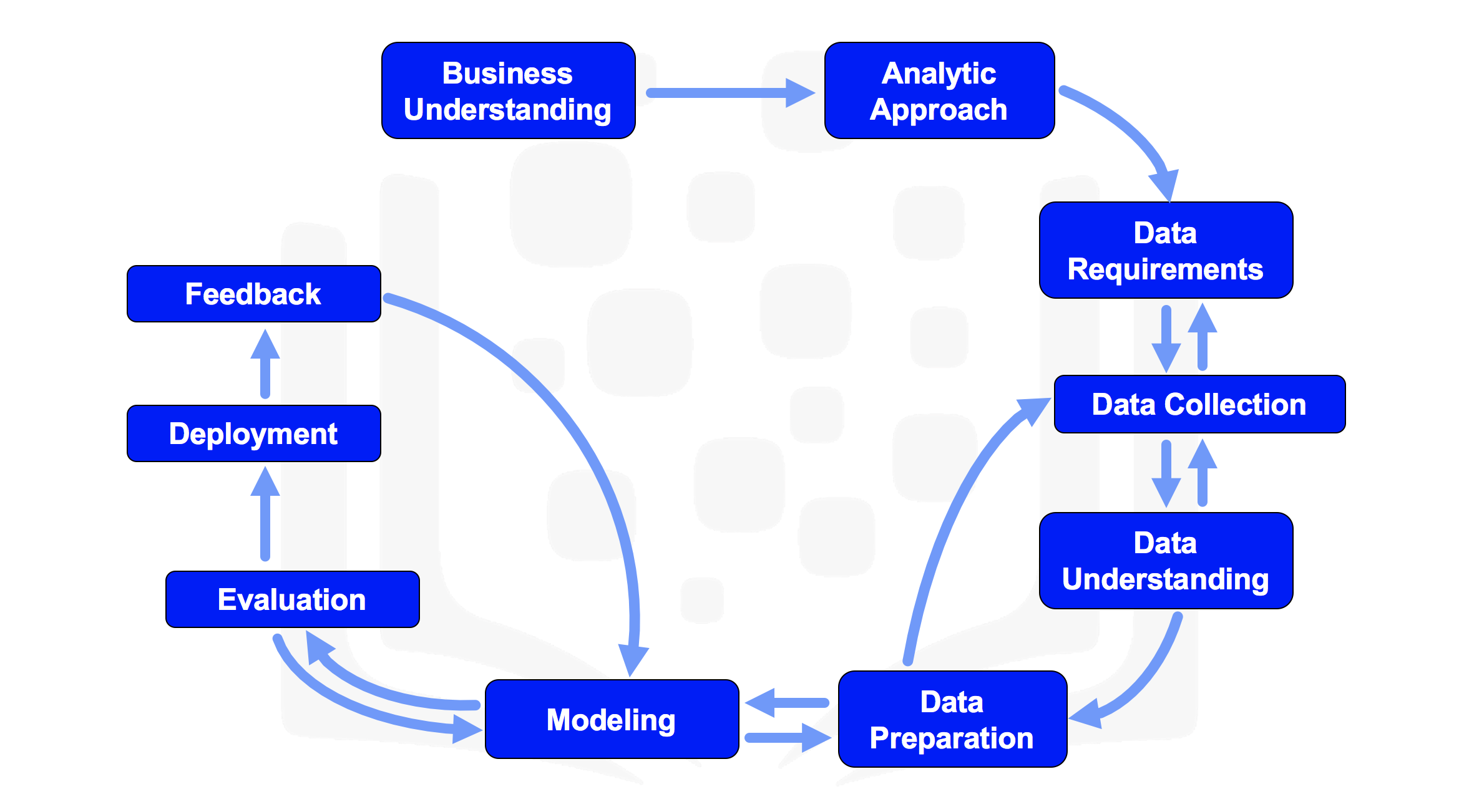
The data science methodology described here is as outlined by John Rollins of IBM
The Methodology can be seen in the following steps
The Questions
The Data Science methodology aims to answer ten main questions
From Problem to Approach
- What is the problem you are trying to solve?
- How can you use data to answer the question?
Working with the Data
- What data do you need to answer the question?>
- Where is the data coming from and how will you get it?
- Is the data that you collected representative of the problem to be solved?
- What additional work is required to manipulate and work with the data
Deriving the Answer
- In what way can the data be visualized to get to the answer that is required?
- Does the model used really answer the initial question or does it need to be adjusted?
- Can you put the model into practice?
- Can you get constructive feedback into answering the question?
Problem and Approach
Business Understanding
What is the problem you are trying to solve?
The firs step in the methodology involves seeking any needed clarification in order to identify what the problem we are trying to solve is as this drives the data we use and the analytical approach that we will go about applying
It is important to seek clarification early on otherwise we can waste time and resources moving in the wrong direction
In order to understand a question, it is important to understand the goal of the person asking the question
Based on this we will break down objectives and prioritize them
Analytic Approach
How can you use data to answer the question?
The second step in the methodology is electing the correct approach involves the specific problem being addressed, this points to the purpose of business understanding and helps us to identify what methods we should use in order to address the problem
Approach to be Used
When we have a strong understanding of the problem, wwe can pick an analytical approach to be used
- Descriptive
- Current Status
- Diagnostic (Statistical Analysis)
- What happened?
- Why is this happening?
- Predictive (Forecasting)
- What if these trends continue?
- What will happen next?
- Prescriptive
- How do we solve it?
Question Types
We have a few different types of questions that can direct our modelling
- Question is to determine probabilities of an action
- Predictive Model
- Question is to show relationships
- Descriptive Model
- Question requires a binary answer
- Classification Model
Machine Learning
Machine learning allows us to identify relationships and trends that cannot otherwise be established
Decision Trees
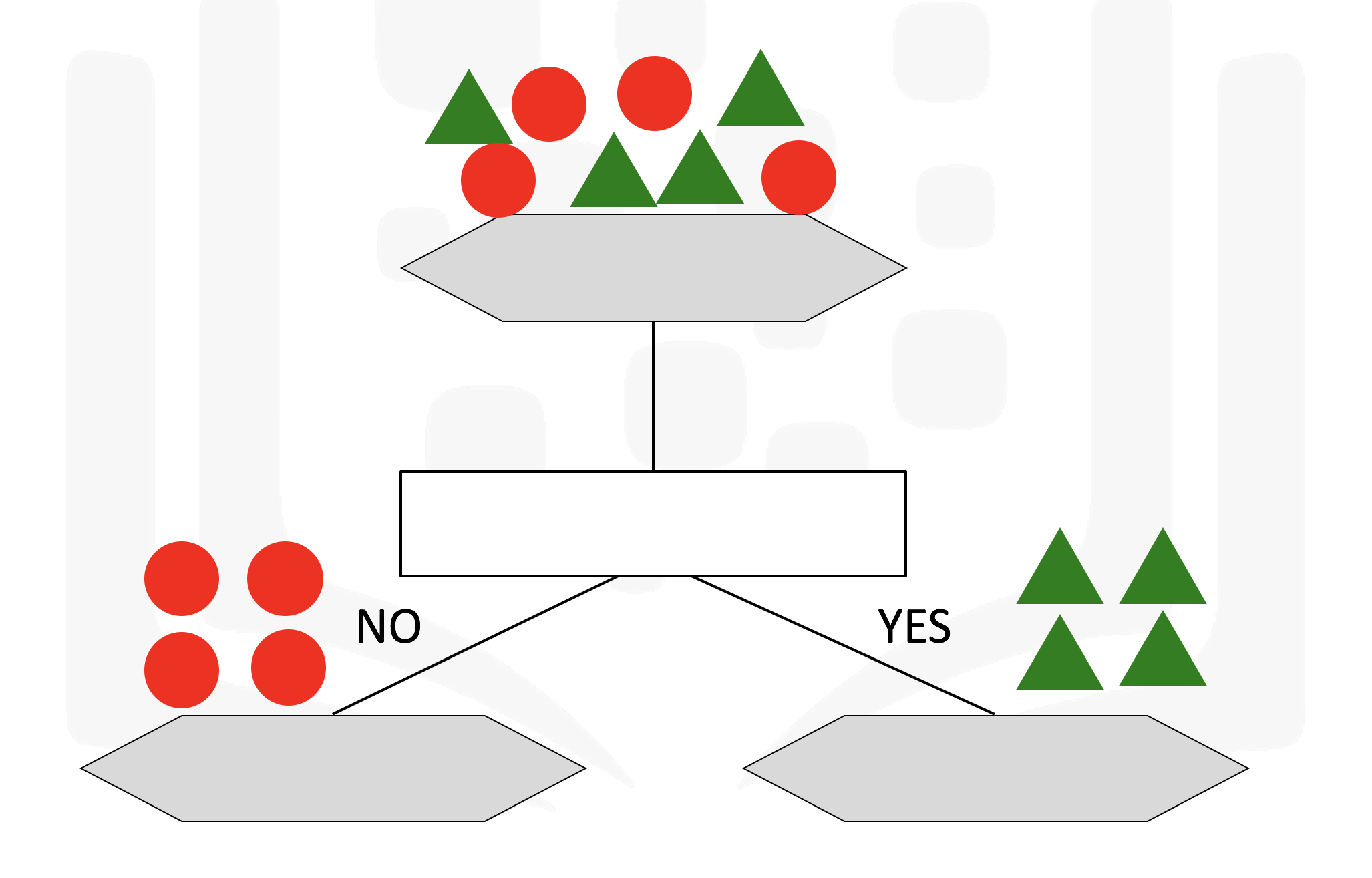
Decision trees are a machine learning algorithm that allow us to classify nodes while also giving us some information as to how the information is classified
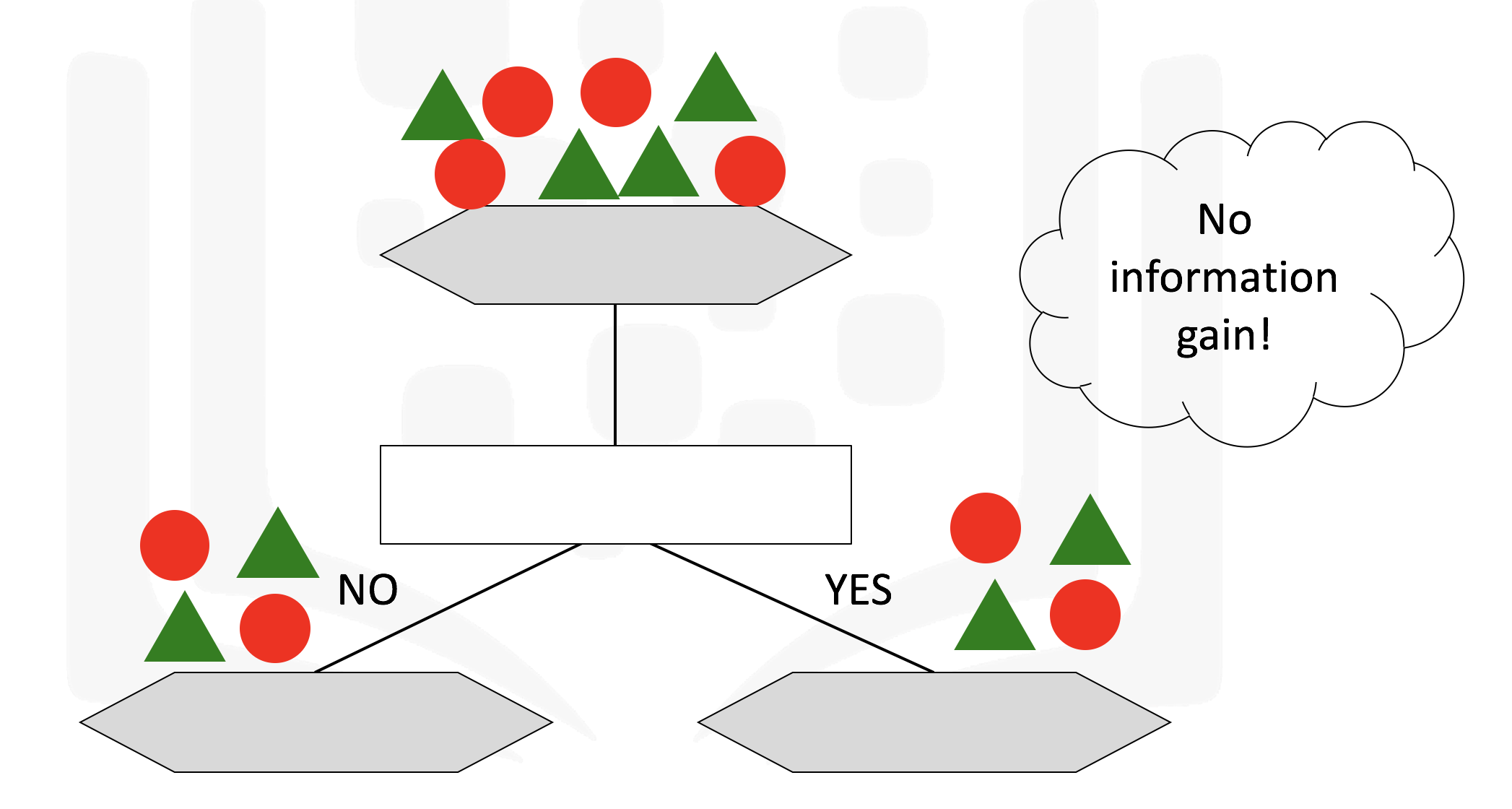
It makes use of a tree structure with recursive partitioning to classify data, predictiveness is based on decrease in entropy - gain in information or impurity
A decision tree for classifying data can result in leaf nodes of varying purity, as seen below which will provide us with different ammounts of information
Some of the characteristics of decision trees are summarized below
| Pros | Cons |
|---|---|
| Easy to interpret | Easy to over or underfit the model |
| Can handle numeric or categorical features | Cannot model feature interaction |
| Can handle missing data | Large trees can be difficult to interpret |
| Uses only the most important features | |
| Can be used on very large or small datasets |
Labs
The Lab notebooks have been added in the labs folder, and are released under the MIT License
The Lab for this section is 1-From-Problem-to-Approach.ipynb
Requirements and Collection
Data Requirements
What data do you need to answer the question?
We need to understand what data is required, how to collect it, and how to transform it to address the problem at hand
It is necessary to identify the data requirements for the initial data collection
We typically make use of the following steps
- Define and select the set of data needed
- Content format and representation of data was defined
- It is important to look ahead when transforming our data to a form that would be most suitable for us
Data Collection
Where is the data coming from and how will you get it?
After the initial data collection has been performed, we look at the data and verify that we have all the data that we need, and the data requirements are revisited in order to define what has not been met or needs to be changed
We then make use of descriptive statistics and visuals in order to define the quality and other aspects of the data and then identify how we can fill in these gaps
Collecting data requires that we know the data source and where to find the required data
Labs
The lab documents for this section are in both Python and R, and can be found in the labs folder as 2-Requirements-to-Collection-py.ipynb and 2-Requirements-to-Collection-R.ipynb
These labs will simply read in a dataset from a remote source as a CSV and display it
Python
In Python we will use Pandas to read data as DataFrames
We can use Pandas to read data into the data frame
1import pandas as pd # download library to read data into dataframe2pd.set_option('display.max_columns', None)3
4recipes = pd.read_csv("https://ibm.box.com/shared/static/5wah9atr5o1akuuavl2z9tkjzdinr1lv.csv")5
6print("Data read into dataframe!") # takes about 30 seconds
Thereafter we can view the dataframe by looking at the first few rows, as well as the dimensions with
1recipes.head()2recipes.shapeR
We do the same aas the above in R as follows
First we download the file from the remote resource
1# click here and press Shift + Enter2download.file("https://ibm.box.com/shared/static/5wah9atr5o1akuuavl2z9tkjzdinr1lv.csv",3              destfile = "/resources/data/recipes.csv", quiet = TRUE)4
5print("Done!") # takes about 30 seconds
Thereafter we can read this into a variable with
1recipes <- read.csv("/resources/data/recipes.csv") # takes 10 secWe can then see the first few rows of data as well as the dimensions with
1head(recipes)2nrow(recipes)3ncol(recipes)Understanding and Preparation
Data Understanding
Is the data that you collected representative of the problem to be solved?
We make use of descriptive statistics to understand the data
We run statistical analyses to learn about the data with means such as such as
- Univariate
- Pairwise
- Histogram
- Mean
- Medium
- Min
- Max
- etc.
We also make use of these to understand data quality and values such as Missing values and Invalid or Misleading values
Data Preparation
What additional work is required to manipulate and work with the data
Data preparation is similar to cleansing data by removing unwanted elements and imperfections, this can take between 70% and 90% of the project time
Transforming data in this phase is the process of turining data into something that would be easier to work with
Some examples of what we need to look out for are
- Invalid values
- Missing data
- Duplicates
- Formatting
Another part of data preparation is feature engineering which is when we use domain knowledge to create features for our predictive models
The data preparation will support the remainder of the project
Labs
The lab documents for this section are in both Python and R, and can be found in the labs folder as 3-Understanding-to-Preparation-py.ipynb and 3-Understanding-to-Preparation-R.ipynb
These labs will continue to analyze the data that was imported from the previous lab
Python
First, we check if the ingredients exist in our dataframe
1ingredients = list(recipes.columns.values)2
3print([match.group(0) for ingredient in ingredients for match in [(re.compile(".*(rice).*")).search(ingredient)] if match])4print([match.group(0) for ingredient in ingredients for match in [(re.compile(".*(wasabi).*")).search(ingredient)] if match])5print([match.group(0) for ingredient in ingredients for match in [(re.compile(".*(soy).*")).search(ingredient)] if match])
Thereafter we can look at our data in order to see if there are any changes that need to be made
1recipes["country"].value_counts() # frequency table2
3# American                   401504# Mexico                      17545# Italian                     17156# Italy                       14617# Asian                       11768# French                       9969# east_asian                   95110# Canada                       77411# korean                       76712# Mexican                      62213# western                      45014# Southern_SoulFood            34615# India                        32416# Jewish                       32017# Spanish_Portuguese           291
From here the following can be seen
- Cuisine is labelled as country
- Cuisine names are not consistent, uppercase, lowercase, etc.
- Some cuisines are duplicates of the country name
- Some cuisines have very few recipes
We can take a few steps to solve these problems
First we fix the Country title to be Cuisine
1column_names = recipes.columns.values2column_names[0] = "cuisine"3recipes.columns = column_names4
5recipes
Then we can make all the names lowercase
1recipes["cuisine"] = recipes["cuisine"].str.lower()Next we correct the mislablled cuisine names
1recipes.loc[recipes["cuisine"] == "austria", "cuisine"] = "austrian"2recipes.loc[recipes["cuisine"] == "belgium", "cuisine"] = "belgian"3recipes.loc[recipes["cuisine"] == "china", "cuisine"] = "chinese"4recipes.loc[recipes["cuisine"] == "canada", "cuisine"] = "canadian"5recipes.loc[recipes["cuisine"] == "netherlands", "cuisine"] = "dutch"6recipes.loc[recipes["cuisine"] == "france", "cuisine"] = "french"7recipes.loc[recipes["cuisine"] == "germany", "cuisine"] = "german"8recipes.loc[recipes["cuisine"] == "india", "cuisine"] = "indian"9recipes.loc[recipes["cuisine"] == "indonesia", "cuisine"] = "indonesian"10recipes.loc[recipes["cuisine"] == "iran", "cuisine"] = "iranian"11recipes.loc[recipes["cuisine"] == "italy", "cuisine"] = "italian"12recipes.loc[recipes["cuisine"] == "japan", "cuisine"] = "japanese"13recipes.loc[recipes["cuisine"] == "israel", "cuisine"] = "jewish"14recipes.loc[recipes["cuisine"] == "korea", "cuisine"] = "korean"15recipes.loc[recipes["cuisine"] == "lebanon", "cuisine"] = "lebanese"16recipes.loc[recipes["cuisine"] == "malaysia", "cuisine"] = "malaysian"17recipes.loc[recipes["cuisine"] == "mexico", "cuisine"] = "mexican"18recipes.loc[recipes["cuisine"] == "pakistan", "cuisine"] = "pakistani"19recipes.loc[recipes["cuisine"] == "philippines", "cuisine"] = "philippine"20recipes.loc[recipes["cuisine"] == "scandinavia", "cuisine"] = "scandinavian"21recipes.loc[recipes["cuisine"] == "spain", "cuisine"] = "spanish_portuguese"22recipes.loc[recipes["cuisine"] == "portugal", "cuisine"] = "spanish_portuguese"23recipes.loc[recipes["cuisine"] == "switzerland", "cuisine"] = "swiss"24recipes.loc[recipes["cuisine"] == "thailand", "cuisine"] = "thai"25recipes.loc[recipes["cuisine"] == "turkey", "cuisine"] = "turkish"26recipes.loc[recipes["cuisine"] == "vietnam", "cuisine"] = "vietnamese"27recipes.loc[recipes["cuisine"] == "uk-and-ireland", "cuisine"] = "uk-and-irish"28recipes.loc[recipes["cuisine"] == "irish", "cuisine"] = "uk-and-irish"29
30recipes
After that we can remove the cuisines with less than 50 recipes
1# get list of cuisines to keep2recipes_counts = recipes["cuisine"].value_counts()3cuisines_indices = recipes_counts > 504
5cuisines_to_keep = list(np.array(recipes_counts.index.values)[np.array(cuisines_indices)])
And then view the number of rows we kepy/removed
1rows_before = recipes.shape[0] # number of rows of original dataframe2print("Number of rows of original dataframe is {}.".format(rows_before))3
4recipes = recipes.loc[recipes['cuisine'].isin(cuisines_to_keep)]5
6rows_after = recipes.shape[0] # number of rows of processed dataframe7print("Number of rows of processed dataframe is {}.".format(rows_after))8
9print("{} rows removed!".format(rows_before - rows_after))
Next we can convert the yes/no fields to be binary
1recipes = recipes.replace(to_replace="Yes", value=1)2recipes = recipes.replace(to_replace="No", value=0)And lastly view our data with
1recipes.head()Next we can Look for recipes that contain rice and soy and wasabi and seaweed
1check_recipes = recipes.loc[2    (recipes["rice"] == 1) &3    (recipes["soy_sauce"] == 1) &4    (recipes["wasabi"] == 1) &5    (recipes["seaweed"] == 1)6]7
8check_recipes
Based on this we can see that not all recipes with those ingredients are Japanese
Now we can look at the frequency of different ingredients in these recipes
1# sum each column2ing = recipes.iloc[:, 1:].sum(axis=0)3# define each column as a pandas series4ingredient = pd.Series(ing.index.values, index = np.arange(len(ing)))5count = pd.Series(list(ing), index = np.arange(len(ing)))6
7# create the dataframe8ing_df = pd.DataFrame(dict(ingredient = ingredient, count = count))9ing_df = ing_df[["ingredient", "count"]]10print(ing_df.to_string())
We can then sort the dataframe of ingredients in descending order
1# define each column as a pandas series2ingredient = pd.Series(ing.index.values, index = np.arange(len(ing)))3count = pd.Series(list(ing), index = np.arange(len(ing)))4
5# create the dataframe6ing_df = pd.DataFrame(dict(ingredient = ingredient, count = count))7ing_df = ing_df[["ingredient", "count"]]8print(ing_df.to_string())
From this we can see that the most common ingredients are Egg, Wheat, and Butter. However we have a lot more American recipes than the others, indicating that our data is skewed towards American ingredients
We can now create a profile for each cuisine in order to see a more representative recipe distribution with
1cuisines = recipes.groupby("cuisine").mean()2cuisines.head()We can then print out the top 4 ingredients of every couisine with the following
1num_ingredients = 4 # define number of top ingredients to print2
3# define a function that prints the top ingredients for each cuisine4def print_top_ingredients(row):5    print(row.name.upper())6    row_sorted = row.sort_values(ascending=False)*1007    top_ingredients = list(row_sorted.index.values)[0:num_ingredients]8    row_sorted = list(row_sorted)[0:num_ingredients]9
10    for ind, ingredient in enumerate(top_ingredients):11        print("%s (%d%%)" % (ingredient, row_sorted[ind]), end=' ')12    print("\n")13
14# apply function to cuisines dataframe15create_cuisines_profiles = cuisines.apply(print_top_ingredients, axis=1)16
17# AFRICAN18# onion (53%) olive_oil (52%) garlic (49%) cumin (42%)19
20# AMERICAN21# butter (41%) egg (40%) wheat (39%) onion (29%)22
23# ASIAN24# soy_sauce (49%) ginger (48%) garlic (47%) rice (41%)25
26# CAJUN_CREOLE27# onion (69%) cayenne (56%) garlic (48%) butter (36%)28
29# CANADIAN30# wheat (39%) butter (38%) egg (35%) onion (34%)
R
First, we check if the ingredients exist in our dataframe
1grep("rice", names(recipes), value = TRUE) # yes as rice2grep("wasabi", names(recipes), value = TRUE) # yes3grep("soy", names(recipes), value = TRUE) # yes as soy_sauceThereafter we can look at our data in order to see if there are any changes that need to be made
1base::table(recipes$country) # frequency table2
3# American                   401504# Mexico                      17545# Italian                     17156# Italy                       14617# Asian                       11768# French                       9969# east_asian                   95110# Canada                       77411# korean                       76712# Mexican                      62213# western                      45014# Southern_SoulFood            34615# India                        32416# Jewish                       32017# Spanish_Portuguese           291
From here the following can be seen
- Cuisine is labelled as country
- Cuisine names are not consistent, uppercase, lowercase, etc.
- Some cuisines are duplicates of the country name
- Some cuisines have very few recipes
We can take a few steps to solve these problems
First we fix the Country title to be Cuisine
1colnames(recipes)[1] = "cuisine"Then we can make all the names lowercase
1recipes$cuisine <- tolower(as.character(recipes$cuisine))2
3recipes
Next we correct the mislablled cuisine names
1recipes$cuisine[recipes$cuisine == "austria"] <- "austrian"2recipes$cuisine[recipes$cuisine == "belgium"] <- "belgian"3recipes$cuisine[recipes$cuisine == "china"] <- "chinese"4recipes$cuisine[recipes$cuisine == "canada"] <- "canadian"5recipes$cuisine[recipes$cuisine == "netherlands"] <- "dutch"6recipes$cuisine[recipes$cuisine == "france"] <- "french"7recipes$cuisine[recipes$cuisine == "germany"] <- "german"8recipes$cuisine[recipes$cuisine == "india"] <- "indian"9recipes$cuisine[recipes$cuisine == "indonesia"] <- "indonesian"10recipes$cuisine[recipes$cuisine == "iran"] <- "iranian"11recipes$cuisine[recipes$cuisine == "israel"] <- "jewish"12recipes$cuisine[recipes$cuisine == "italy"] <- "italian"13recipes$cuisine[recipes$cuisine == "japan"] <- "japanese"14recipes$cuisine[recipes$cuisine == "korea"] <- "korean"15recipes$cuisine[recipes$cuisine == "lebanon"] <- "lebanese"16recipes$cuisine[recipes$cuisine == "malaysia"] <- "malaysian"17recipes$cuisine[recipes$cuisine == "mexico"] <- "mexican"18recipes$cuisine[recipes$cuisine == "pakistan"] <- "pakistani"19recipes$cuisine[recipes$cuisine == "philippines"] <- "philippine"20recipes$cuisine[recipes$cuisine == "scandinavia"] <- "scandinavian"21recipes$cuisine[recipes$cuisine == "spain"] <- "spanish_portuguese"22recipes$cuisine[recipes$cuisine == "portugal"] <- "spanish_portuguese"23recipes$cuisine[recipes$cuisine == "switzerland"] <- "swiss"24recipes$cuisine[recipes$cuisine == "thailand"] <- "thai"25recipes$cuisine[recipes$cuisine == "turkey"] <- "turkish"26recipes$cuisine[recipes$cuisine == "irish"] <- "uk-and-irish"27recipes$cuisine[recipes$cuisine == "uk-and-ireland"] <- "uk-and-irish"28recipes$cuisine[recipes$cuisine == "vietnam"] <- "vietnamese"29
30recipes
After that we can remove the cuisines with less than 50 recipes
1# sort the table of cuisines by descending order2# get cuisines with >= 50 recipes3filter_list <- names(t[t >= 50])4
5filter_list
And then view the number of rows we kept/removed
1# sort the table of cuisines by descending order2t <- sort(base::table(recipes$cuisine), decreasing = T)3
4t
Next we convert all the columns into factors for classification later
1recipes[,names(recipes)] <- lapply(recipes[,names(recipes)], as.factor)2
3recipes
We can look at the structure of our dataframe as
1str(recipes)Now we can look at which recipes contain rice and soy_sauce and wasabi and seaweed
1check_recipes <- recipes[2    recipes$rice == "Yes" &3    recipes$soy_sauce == "Yes" &4    recipes$wasabi == "Yes" &5    recipes$seaweed == "Yes",6]7
8check_recipes
We can count the ingredients across all recipes with
1# sum the row count when the value of the row in a column is equal to "Yes" (value of 2)2ingred <- unlist(3            lapply( recipes[, names(recipes)], function(x) sum(as.integer(x) == 2))4            )5
6# transpose the dataframe so that each row is an ingredient7ingred <- as.data.frame( t( as.data.frame(ingred) ))8
9ing_df <- data.frame("ingredient" = names(ingred),10                     "count" = as.numeric(ingred[1,])11                    )[-1,]12
13ing_df
We can next count the total ingredients and sort that in descending order
1ing_df_sort <- ing_df[order(ing_df$count, decreasing = TRUE),]2rownames(ing_df_sort) <- 1:nrow(ing_df_sort)3
4ing_df_sort
We can then create a profile for each cuisine as we did previously
1# create a dataframe of the counts of ingredients by cuisine, normalized by the number of2# recipes pertaining to that cuisine3by_cuisine_norm <- aggregate(recipes,4                        by = list(recipes$cuisine),5                        FUN = function(x) round(sum(as.integer(x) == 2)/6                                                length(as.integer(x)),4))7# remove the unnecessary column "cuisine"8by_cuisine_norm <- by_cuisine_norm[,-2]9
10# rename the first column into "cuisine"11names(by_cuisine_norm)[1] <- "cuisine"12
13head(by_cuisine_norm)
We can then print out the top 4 ingredients for each recipe with
1for(nation in by_cuisine_norm$cuisine){2 x <- sort(by_cuisine_norm[by_cuisine_norm$cuisine == nation,][-1], decreasing = TRUE)3 cat(c(toupper(nation)))4 cat("\n")5 cat(paste0(names(x)[1:4], " (", round(x[1:4]*100,0), "%) "))6 cat("\n")7 cat("\n")8}Modeling and Evaluation
Modeling
In what way can the data be visualized to get to the answer that is required?
Modeling is the stage in which the Data Scientist
Data modeling either tries to get to a predictive or descriptive model
Data scientists use a training set for predictive modeling, this is historical data that acts as a way to test that the data we are using is suitable for the problem we are tryig to solve
Evaluation
Does the model used really answer the initial question or does it need to be adjusted?
A model evaluation goes hand in hand with model building, model building and evaluation are done iteratively
This is done before the model is deployed in order to verify that the model answers our questions and the quality meets our standard
Two phases are considered when evaluating a model
- Diagnostic Measures
- Predictive
- Descriptive
- Statistical Significance
We can make use of the ROC curve to evaluate models and determine the optimal model for a binary classification model by plotting the True-Positive vs False-Positive rate for the model
Labs
The lab documents for this section are in both Python and R, and can be found in the labs folder as 4-Modeling-to-Evaluation-py.ipynb and 4-Modeling-to-Evaluation-R.ipynb
These labs will continue from where the last lab left off and build a decision Tree Model for the recipe data
Python
First we will need to import some libraries for modelling
1# import decision trees scikit-learn libraries2%matplotlib inline3from sklearn import tree4from sklearn.metrics import accuracy_score, confusion_matrix5
6import matplotlib.pyplot as plt7
8!conda install python-graphviz --yes9import graphviz10
11from sklearn.tree import export_graphviz12
13import itertools
We will make use of a decision tree called bamboo_tree which will be used to classify between Korean, Japanese, Chinese, Thai, and Indian Food
The following code will create our decision tree
1# select subset of cuisines2asian_indian_recipes = recipes[recipes.cuisine.isin(["korean", "japanese", "chinese", "thai", "indian"])]3cuisines = asian_indian_recipes["cuisine"]4ingredients = asian_indian_recipes.iloc[:,1:]5
6bamboo_tree = tree.DecisionTreeClassifier(max_depth=3)7bamboo_tree.fit(ingredients, cuisines)8
9print("Decision tree model saved to bamboo_tree!")
Thereafter we can plot the decision tree with
1export_graphviz(bamboo_tree,2                feature_names=list(ingredients.columns.values),3                out_file="bamboo_tree.dot",4                class_names=np.unique(cuisines),5                filled=True,6                node_ids=True,7                special_characters=True,8                impurity=False,9                label="all",10                leaves_parallel=False)11
12with open("bamboo_tree.dot") as bamboo_tree_image:13    bamboo_tree_graph = bamboo_tree_image.read()14graphviz.Source(bamboo_tree_graph)
Now we can go back and rebuild our model, however this time retaining some data so we can evaluate the model
1bamboo = recipes[recipes.cuisine.isin(["korean", "japanese", "chinese", "thai", "indian"])]2bamboo["cuisine"].value_counts()We can use 30 values as our sample size
1# set sample size2sample_n = 303# take 30 recipes from each cuisine4random.seed(1234) # set random seed5bamboo_test = bamboo.groupby("cuisine", group_keys=False).apply(lambda x: x.sample(sample_n))6
7bamboo_test_ingredients = bamboo_test.iloc[:,1:] # ingredients8bamboo_test_cuisines = bamboo_test["cuisine"] # corresponding cuisines or labels
We can verify that we have 30 recipes from each cuisine
1# check that we have 30 recipes from each cuisine2bamboo_test["cuisine"].value_counts()We can now separate our data in to a test and training set
1bamboo_test_index = bamboo.index.isin(bamboo_test.index)2bamboo_train = bamboo[~bamboo_test_index]3
4bamboo_train_ingredients = bamboo_train.iloc[:,1:] # ingredients5bamboo_train_cuisines = bamboo_train["cuisine"] # corresponding cuisines or labels6
7bamboo_train["cuisine"].value_counts()
And then train our model again
1bamboo_train_tree = tree.DecisionTreeClassifier(max_depth=15)2bamboo_train_tree.fit(bamboo_train_ingredients, bamboo_train_cuisines)3
4print("Decision tree model saved to bamboo_train_tree!")
We can then view our tree as before
1export_graphviz(bamboo_train_tree,2                feature_names=list(bamboo_train_ingredients.columns.values),3                out_file="bamboo_train_tree.dot",4                class_names=np.unique(bamboo_train_cuisines),5                filled=True,6                node_ids=True,7                special_characters=True,8                impurity=False,9                label="all",10                leaves_parallel=False)11
12with open("bamboo_train_tree.dot") as bamboo_train_tree_image:13    bamboo_train_tree_graph = bamboo_train_tree_image.read()14graphviz.Source(bamboo_train_tree_graph)
If you run this you will see that the new tree is more complex than the last one due to it having fewer data points to work with (I did not put it here because it renders very big in the plot)
Next we can test our model based on the Test Data
1bamboo_pred_cuisines = bamboo_train_tree.predict(bamboo_test_ingredients)We can then create a confusion matrix to see how well the tree does
1test_cuisines = np.unique(bamboo_test_cuisines)2bamboo_confusion_matrix = confusion_matrix(bamboo_test_cuisines, bamboo_pred_cuisines, test_cuisines)3title = 'Bamboo Confusion Matrix'4cmap = plt.cm.Blues5
6plt.figure(figsize=(8, 6))7bamboo_confusion_matrix = (8    bamboo_confusion_matrix.astype('float') / bamboo_confusion_matrix.sum(axis=1)[:, np.newaxis]9    ) * 10010
11plt.imshow(bamboo_confusion_matrix, interpolation='nearest', cmap=cmap)12plt.title(title)13plt.colorbar()14tick_marks = np.arange(len(test_cuisines))15plt.xticks(tick_marks, test_cuisines)16plt.yticks(tick_marks, test_cuisines)17
18fmt = '.2f'19thresh = bamboo_confusion_matrix.max() / 2.20for i, j in itertools.product(range(bamboo_confusion_matrix.shape[0]), range(bamboo_confusion_matrix.shape[1])):21    plt.text(j, i, format(bamboo_confusion_matrix[i, j], fmt),22             horizontalalignment="center",23             color="white" if bamboo_confusion_matrix[i, j] > thresh else "black")24
25plt.tight_layout()26plt.ylabel('True label')27plt.xlabel('Predicted label')28
29plt.show()
The rows on a confusion matrix epresent the actual values, and the rows are the predicted values
The resulting confusion matrix can be seen below
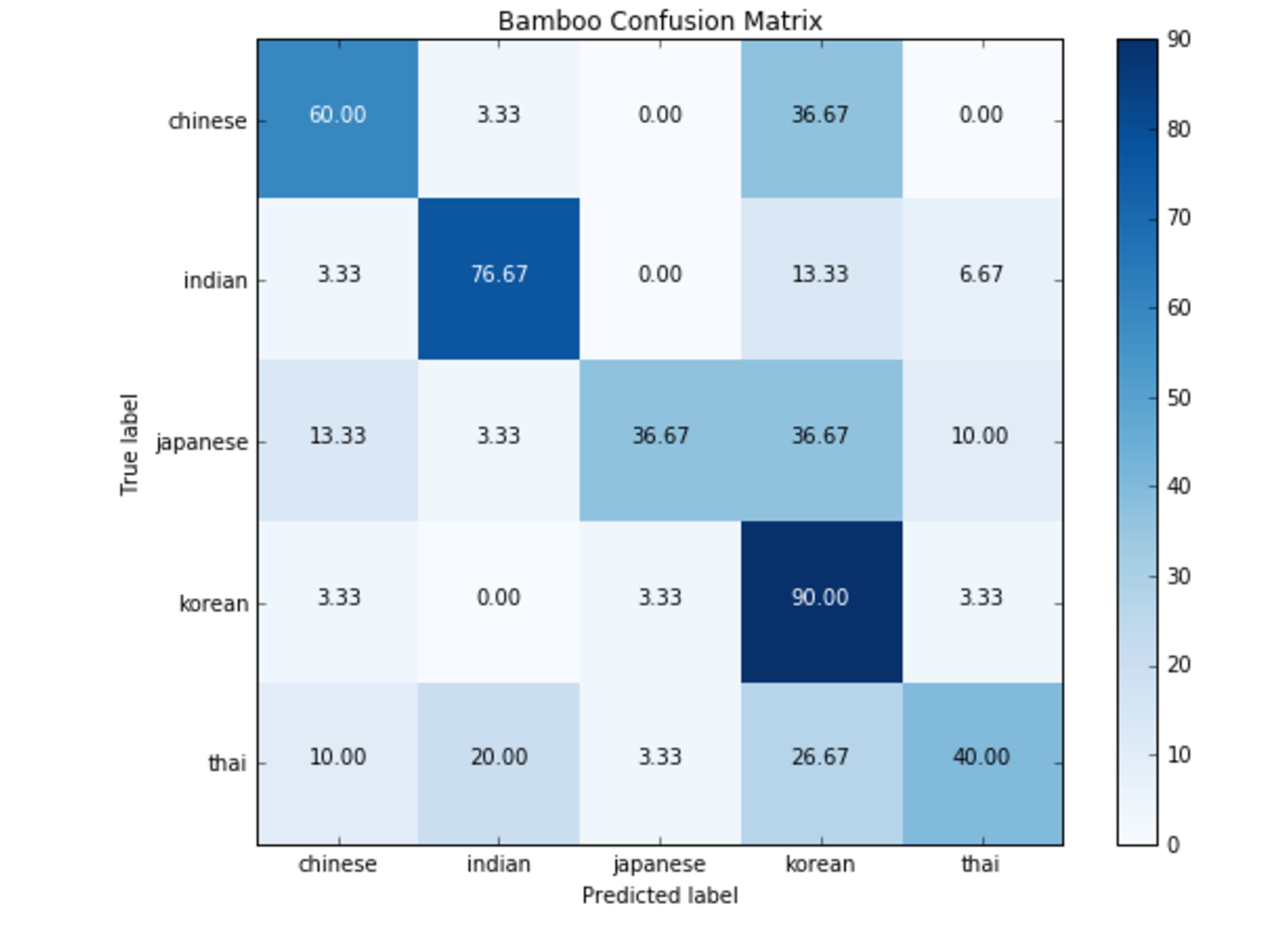
The squares along the top-left to bottom-right diagonal are those that the model correctly classified
R
We can follow a similar process as above using R
First we import the libraries we will need to build our decision trees as follows
1# load libraries2library(rpart)3
4if("rpart.plot" %in% rownames(installed.packages()) == FALSE) {install.packages("rpart.plot",5    repo = "http://mirror.las.iastate.edu/CRAN/")}6library(rpart.plot)7
8print("Libraries loaded!")
Thereafter we can train our model using our data with
1# select subset of cuisines2cuisines_to_keep = c("korean", "japanese", "chinese", "thai", "indian")3cuisines_data <- recipes[recipes$cuisine %in% cuisines_to_keep, ]4cuisines_data$cuisine <- as.factor(as.character(cuisines_data$cuisine))5
6bamboo_tree <- rpart(formula=cuisine ~ ., data=cuisines_data, method ="class")7
8print("Decision tree model saved to bamboo_tree!")
And view it with the following
1# plot bamboo_tree2rpart.plot(bamboo_tree, type=3, extra=2, under=TRUE, cex=0.75, varlen=0, faclen=0, Margin=0.03)
Now we can redefine our dataframe to only include the Asian and Indian cuisine
1bamboo <- recipes[recipes$cuisine %in% c("korean", "japanese", "chinese", "thai", "indian"),]And take a sample of 30 for our test set from each cuisine
1# take 30 recipes from each cuisine2set.seed(4) # set random seed3korean <- bamboo[base::sample(which(bamboo$cuisine == "korean") , sample_n), ]4japanese <- bamboo[base::sample(which(bamboo$cuisine == "japanese") , sample_n), ]5chinese <- bamboo[base::sample(which(bamboo$cuisine == "chinese") , sample_n), ]6thai <- bamboo[base::sample(which(bamboo$cuisine == "thai") , sample_n), ]7indian <- bamboo[base::sample(which(bamboo$cuisine == "indian") , sample_n), ]8
9# create the dataframe10bamboo_test <- rbind(korean, japanese, chinese, thai, indian)
Thereafter we can create our training set with
1bamboo_train <- bamboo[!(rownames(bamboo) %in% rownames(bamboo_test)),]2bamboo_train$cuisine <- as.factor(as.character(bamboo_train$cuisine))And verify that we have correctly removed the 30 elements from each revipe
1base::table(bamboo_train$cuisine)Next we can train our tree and plot it
1bamboo_train_tree <- rpart(formula=cuisine ~ ., data=bamboo_train, method="class")2rpart.plot(bamboo_train_tree, type=3, extra=0, under=TRUE, cex=0.75, varlen=0, faclen=0, Margin=0.03)It can be seen that by removing elements we get a more complex decision tree, this is the same as in the Python case

We can then view the confusion matrix as follows
1bamboo_confusion_matrix <- base::table(2    paste(as.character(bamboo_test$cuisine),"_true", sep=""),3    paste(as.character(bamboo_pred_cuisines),"_pred", sep="")4)5
6round(prop.table(bamboo_confusion_matrix, 1)*100, 1)
Which will result in
1 chinese_pred indian_pred japanese_pred korean_pred thai_pred2 chinese_true 60.0 0.0 3.3 36.7 0.03 indian_true 0.0 90.0 0.0 10.0 0.04 japanese_true 20.0 3.3 33.3 40.0 3.35 korean_true 6.7 0.0 16.7 76.7 0.06 thai_true 3.3 20.0 0.0 33.3 43.3Deployment and Feedback
Deployment
Can you put the model into practice?
The key to making your model relevant is making the stakeholders familiar with the solution developed
When the model is evaluated and we are confident in the model we deploy it, typically first to a small set of users to put it through practical tests
Deployment also consists of developing a suitable method to enable our users to interact with and use the model as well as looking to ways to improve the model with a feedback system
Feedback
Can you get constructive feedback into answering the question?
User feedback helps us to refine and assess the model’s performance and impact, and based on this feedback making changes to make the model
Once the model is deployed we can make use of feedback and experience with the model to refine the model or incorporate different data into it that we had not initally considered